Physics Informed Neural Networks in Engineering

Physics-informed neural networks (PINNs) are a framework for training artificial neural networks, particularly deep neural networks, to solve complex problems. Physical laws govern those problems; for instance, consider fluid dynamics, heat transfer, or electromagnetism.

PINNs are specifically designed for modeling real-world physical processes and systems by incorporating physical laws directly into the learning process.

Partial differential equations (PDEs) offer the mathematical description of the governing laws. In PINNs, those differential equations are incorporated into the neural network’s loss function. PINNs leverage the universal approximation theorem and the high expressivity of deep neural networks to approximate solutions of partial differential equations (PDEs).

PINNs do not directly solve the differential equations. Instead, PINNs embed prior knowledge described by differential equations into neural networks. We constrain those neural networks to produce outputs that satisfy the governing laws and the available input data. Mathematically, this is done by minimizing a “loss function”.

The "loss function" of PINNs consists of several terms: a physics-informed term and, optionally, terms that evaluate the error between the network's predictions and values prescribed by initial and/or boundary data. The loss function penalizes deviations from the physical equations and other conditions.

In summary, a PINN is a constrained optimization problem that seeks to reduce mismatches. The solutions produced by physically informed neural networks (PINNs) are:

• characteristically data-driven, like in modern AI
• physically consistent, even with sparse input data

This physics-driven, data-supported approach is intended to bridge the gap between traditional numerical methods and pure data-driven AI. Learn more about the major fields of Artificial Intelligence.

Highlights:

• The innovation of physics-informed neural networks lies in their ability to integrate physical laws described by differential equations into their loss functions to guide learning.
• This approach transforms how deep neural network learning models handle problems in physics and engineering by enforcing adherence to underlying physical laws during training.
• PINNs work by incorporating physical laws directly into deep neural network architectures, enabling the modeling of complex physical systems and processes.
• Typically, neural networks require massive datasets and are purely data-driven
• PINNs thrive on less data because they incorporate physical constraints. This distinction makes physics-informed deep learning specifically valuable in applications where obtaining comprehensive measured data can be economically or technically challenging.
• The integration of prior knowledge into the learning process enhances the accuracy and robustness of model predictions while maintaining physical consistency across the entire computational domain.
• First introduced in 2017, PINNs have since seen many variations, including those compatible with different neural network architectures, such as graph neural networks and Fourier neural operators.

Follow us on the journey about PINNs:

• The Basics: Differential Equations in Engineering
• The Mechanics of Physics-Informed Neural Networks
• Advantages and Key Capabilities
• Applications Across Engineering Domains
• The Emerging Role of Geometric Deep Learning
• Detailed Applications in Specialized Fields
• What Are the Challenges and Limitations of Physics-Informed Neural Networks
• Use Cases
• Future Directions and Research Frontiers
• Getting Started with PINNs: Practical Checklist

(Note: The underlined technical terms with a † symbol will lead the reader to a short Technical Vocabulary at the bottom of the article)

The Basics: Differential Equations in Engineering

Before tackling the advanced mechanics of PINNs, let us introduce the core mathematical tools they rely on: differential equations. These are fundamental in engineering and physics because they describe how physical quantities change with respect to one or more independent variables.

Imagine tracking the temperature along a heated metal rod or the velocity of air flowing around a wing. In all these cases, the quantity of interest does not remain constant: it varies either in space or in time, or in both. Differential equations provide a precise way to express these variations.

• Ordinary Differential Equations (ODEs) describe how a quantity changes with respect to a single variable (for instance, time t), using ordinary derivatives d/dt. Example: exponential growth dy/dt = ky from an initial conditiony₀, with solution: y(t)= y₀ eᵏᵗ.
• Partial Differential Equations (PDEs) involve functions of multiple variables (space and time) and their partial derivatives ∂/∂x, ∂/∂y, ∂/∂z, ∂/∂t. They model distributed systems across domains Ω.The symbol ∇ is a compact vector operator: ∇ = (∂/∂x, ∂/∂y, ∂/∂z). For instance
  • ∇ f = gradient of f, i.e., vector of directional rates: (∂u/∂x, ∂u/∂y, ∂u/∂z),
  • ∇ ·v = divergence (scalar measuring outflow),
  • ∇²u = (∇ ·∇ u = ∂²u/∂x² + ∂²u/∂y² + ∂²u/∂z²) is the Laplacian and measures diffusion

Three Famous Partial Differential Equations for Engineers

• The Heat Equation
• The Wave Equation
• The Navier–Stokes Equations

We will review below three major PDEs that are directly relevant to engineers and PINN approaches.

The Heat Equation

The heat equation describes the diffusion of temperature T(x,t) in a solid or fluid at rest. The parameter α is the thermal diffusivity. Recall from the previous section that ∇² is the Laplacian operator associated with diffusion.

∂T/∂t = α ∇² T

The Wave Equation

In acoustics and electromagnetics, the wave equation models vibrating strings, sound waves, or electromagnetic fields. The field u(x, t) represents the wave amplitude, and c is the wave propagation speed.

∂²u/∂t² = c² ∇²u

The Navier–Stokes Equations

In fluid mechanics, the Navier–Stokes equations govern the motion of viscous fluids.

The unknowns are the velocity field u(x, t) and the pressure p(x, t), with ρ the fluid density and μ the dynamic viscosity. The nonlinearity arises from the convective term u·∇u, which renders the equations analytically intractable except in a few exceptional cases.

ρ (∂u/∂t + u·∇ u) = −∇p + μ ∇²u + f

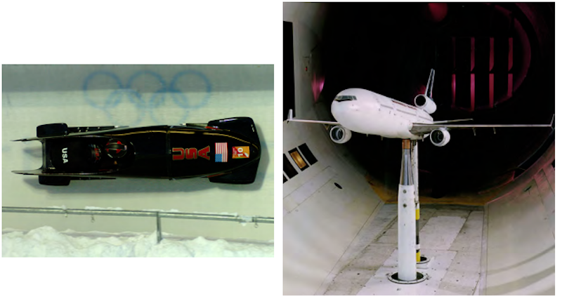
Engineers need to solve them over a spatial domain Ω, subject to appropriate boundary conditions on ∂Ω and initial conditions. Ω can be, for instance, the volume of air in a wind tunnel around a car, bobsled racer, airplane, or wind turbine, and ∂Ω the walls/inlet /outlet of the wind tunnel.

The Mechanics of Physics-Informed Neural Networks

PINNs are not part of an “everyday AI” like natural language processing ChatGPT, but are strongly related to Engineering and Physics. Read a thought leader’s insights on AI and Engineering experience.

PINNs have the following key components:

• a neural network for solutions,
• automatic differentiation for derivatives,
• a hybrid loss that balances data and physics
• a training process for optimization.

Each of those components is crucial for physics-informed learning, especially when addressing problems governed by PDEs and ODEs.

What Are Neural Networks?

Neural networks are computational models loosely inspired by the human brain, built to detect patterns and learn complex mappings from data.

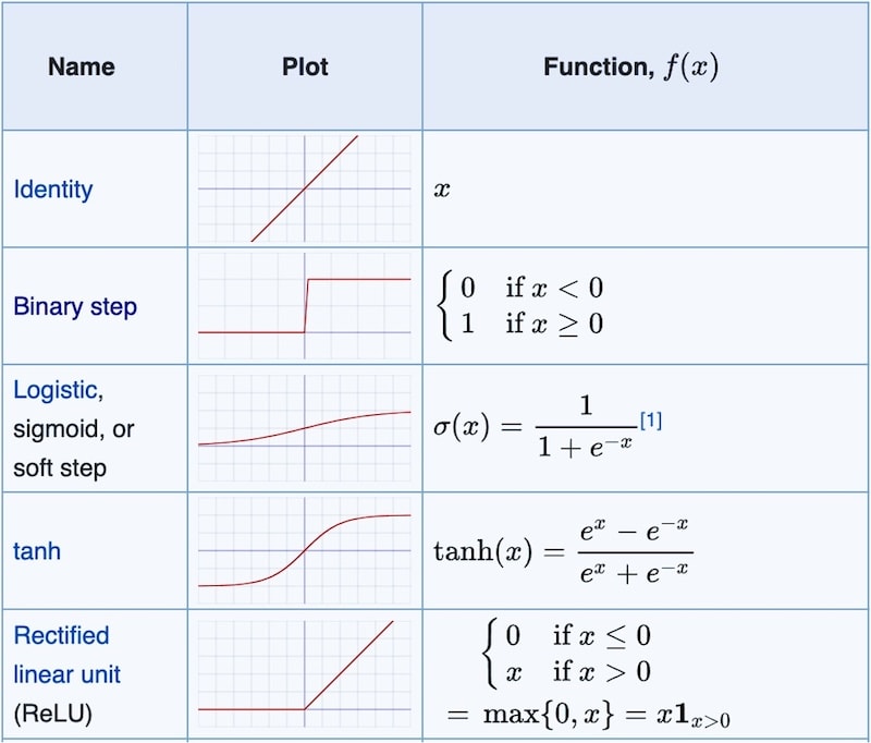
• The basic unit of a neural network is the artificial neuron. The artificial neuron is a simple computational node that takes multiple inputs, computes a weighted sum, adds a bias, and applies a nonlinear activation function to produce an output.

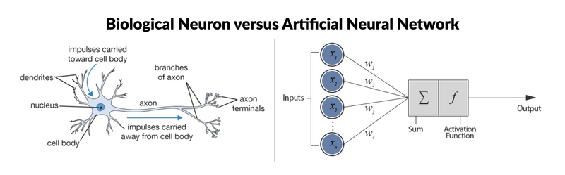
• In plain mathematical terms, if wᵢ are the weights, xᵢ the inputs, b a bias term, and σ the activation function. For example, ReLU: (Rectified Linear Unit) with σ*(z) = max(0, z)*), the output is σ(z), where inputs, weights, and bias are combined as

z = ∑ᵢ (wᵢ xᵢ) + b

• Modern artificial neurons are organized into layers - hence the "deep" in “deep learning."
• An input layer receives data (such as spatial coordinates or sensor readings)
• One or more hidden layers perform successive transformations
• An output layer produces predictions (e.g., temperature or velocity fields)
• During training, millions of weights wᵢ and biases b (collectively known as the model parameters) are adjusted based on data to approximate highly complex, nonlinear relationships. These model parameters are tuned to best fit the data and physical constraints. Once further training no longer reduces the loss or validation error within predefined tolerances, the parameters are fixed, and the network is considered trained.

What are the KPIs for Network Training?

Typical measures of error are the following (MSE, RMSE, MAE, R², Relative / Normalized Error):

• Mean Squared Error (MSE)
• MSE = (1/N) ∑ᵢ (yᵢ − ŷᵢ)²
• Penalizes large errors; standard for regression.
• Root Mean Squared Error (RMSE)
• RMSE = √MSE
• Same units as the target variable.
• Mean Absolute Error (MAE)
• MAE = (1/N) ∑ᵢ |yᵢ − ŷᵢ|
• Less sensitive to outliers than MSE.
• Coefficient of Determination (R²)
• R² = 1 − ∑ᵢ (yᵢ − ŷᵢ)² / ∑ᵢ (yᵢ − ȳ)²
• Measures explained variance (R²=1 → perfect fit).
• Relative / Normalized Error
• e.g. ‖y − ŷ‖₂ / ‖y‖₂
• Useful when comparing across scales.

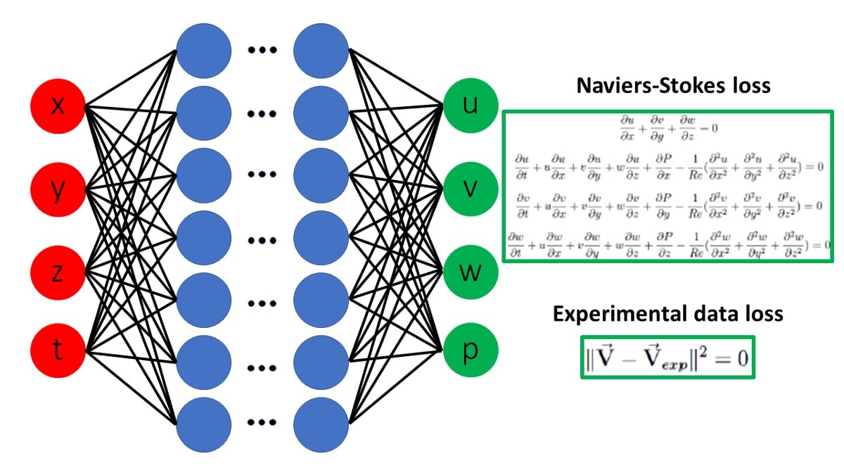
Neural Network as Function Approximator

PINNs exploit the universal approximation property of neural networks: with sufficient width and/or depth, a network can approximate arbitrary continuous functions on compact domains.

In this framework, the neural network represents the unknown solution field of a PDE, mapping input coordinates (space and time) to physical quantities such as velocity, pressure, temperature, or displacement.

Mathematical Formulation

Consider a PDE of the form:

𝓕 [u(x, t)] = f(x, t) where 𝓕 denotes a (possibly nonlinear) differential operator like the ones we saw in the previous chapter.

The neural network u(x, t; θ) is used as a parametric Ansatz for the solution, seeking an approximation

u(x, t) ≈ û(x, t; θ*)

where θ* are the parameters that minimize the physics-informed loss function.

The parameters θ (weights and biases) are optimized during training, enabling the network to represent a continuous solution across spatial and temporal domains while satisfying the governing physical laws.

PINNs as Neural Fields

Unlike finite element or finite difference methods, which require structured grids and discretization, PINNs can be viewed as neural fields. They process continuous spatial and temporal coordinates and output continuous solutions to differential equations.

Thus, the function û(x, t; θ*) can be evaluated at any point without restriction to grid nodes; network functions are considered as a mesh-free alternative to traditional approaches for solving differential equations, allowing for direct application where the boundary ∂Ω of the domain Ω may be highly irregular or time-dependent.

Automatic Differentiation in PINNs

PINNs employ automatic differentiation through backpropagation to compute derivatives of neural network outputs with respect to inputs. For example, innovations in designing a battery cooling plate often rely on advanced simulations and optimization strategies that can leverage such neural network techniques.

The backpropagation algorithm recursively applies the chain rule from outputs to inputs, computing gradients of loss Lwith respect to network parameters θ:

∂L/∂θᵢ = ∂L/∂y · ∂y/∂θᵢ

This enables efficient, exact evaluation of θ-gradients in deep neural network architectures. It yields machine-precision derivatives, essential for nonlinear and higher-order PDEs. Otherwise, small derivative errors accumulate, leading to physically inconsistent solutions.

PDE Residual Evaluation

The automatically differentiated quantities are directly substituted into the governing laws to assemble the differential operators.

• The physics-informed loss evaluates the PDE residual, or the degree to which the PDE is violated at a given point.
• The evaluation is performed at the selected discrete locations within the domain where the PDE is enforced, known as collocation points.
• Because derivatives are extracted from the computational graph, the network enforces differential equation constraints without explicit domain discretization or mesh-based numerical differentiation.

Hybrid Loss Function Architecture

The total loss function combines two components:

• Physics loss (PDE residual): Penalizes violations of the governing PDE at collocation points, enforcing conservation laws and fundamental principles encoded in the differential equations. This term ensures physical laws are respected throughout the domain.
• Data loss: Penalizes mismatches between network predictions and observed measurements at specific locations. Typically computed as mean squared error (MSE), this term ensures the training process respects experimental or simulation data when available. The data-loss weight must be carefully tuned to capture genuine physical trends without overfitting to measurement noise.

Practical Considerations

• PINNs often require careful loss-function tuning to balance data fidelity with physics-based constraints, which can complicate training.
• Integrating complex physical laws requires precise formulations of loss functions that accurately capture the governing laws of the system.

Training Process and Optimization

The network parameters θ are optimized to minimize the combined loss function L

L = L_data + λ·L_physics

The parameter λ controls the trade-off between fitting observed data and enforcing physics constraints. PINNs can be trained using optimization algorithms to iteratively update the neural network parameters until the value of a specified physics-informed loss function decreases to an acceptable level.

This optimization simultaneously approximates the PDE solution and infers underlying physics from sparse measurements. The dual objectives create competing gradients: fitting the data may violate physical constraints, while strictly enforcing physical constraints may overfit to noisy measurements. During training, PINNs balance fitting the given measurements with the underlying physical process.

Training efficiency depends critically on optimizer selection.

• First-order methods like Adam† handle large parameter spaces (10⁵-10⁶ weights) but converge slowly near minima.
• Second-order methods like L-BFGS† achieve superior convergence when the Hessian† is well-conditioned, but become prohibitively expensive for high-dimensional problems. Hybrid strategies that switch from Adam to L-BFGS after initial descent often work best.

Learning rate scheduling† must account for the multi-term loss structure.

Standard decay schedules designed for pure data fitting can prematurely reduce step sizes before physics residuals converge.

Adaptive weighting schemes that gradually increase λ during training (“curriculum learning”) or dynamically adjust loss term coefficients based on gradient magnitudes help balance competing objectives.

Distribution of Collocation Points

The distribution of collocation points profoundly affects solution quality.

• Uniform sampling wastes computation in smooth regions and under-resolves areas with steep gradients or boundary layers.
• Adaptive sampling, which concentrates points where |𝓕[û]| exceeds a threshold, can improve convergence by 2–5× in practice.
• Residual-based Adaptive Refinement (RAR) periodically redistributes points to maintain approximately uniform physics residuals across the domain, ε_i ≈ ε_target.

Pathological Conditioning

The loss landscape can become pathologically conditioned when the physics and data terms operate at very different scales. This happens because the gradients of the loss L with respect to the network parameters θ may differ by orders of magnitude, i.e., in math:

∂L_physics/∂θ >> ∂L_data/∂θ

As a consequence, training either ignores data or vice versa. Careful weight initialization and gradient normalization techniques mitigate these issues, but don’t eliminate them.

In summary, PINNs can be trained using optimization algorithms to iteratively update the neural network parameters until the value of a specified, physics-informed loss function decreases to an acceptable level.

‍

Advantages and Key Capabilities

PINNs offer advantages over both classical numerical methods and pure data-driven approaches. They are particularly effective for modeling complex physical systems governed by high-dimensional and nonlinear partial differential equations. The combination of physical constraints and learning flexibility creates capabilities that prove valuable in engineering contexts where data is limited and problems are complex. Additionally, the network structures of PINNs can be designed or adapted to reflect the underlying physical laws and parameter relationships, improving interpretability and physical consistency.

Data Efficiency and Regularization

One of the most compelling advantages of physics-informed neural networks is their ability to learn accurate solutions even from limited data, thanks to the incorporation of physical laws.

Key aspects include:

• Data efficiency:
• Physics acts as a strong regularizer, preventing unrealistic solutions even with limited sensor data.
• Traditional deep learning often requires massive datasets to generalize well.
• Physical constraints guide learning:
• Incorporating laws like conservation of mass, energy, and momentum reduces the network’s hypothesis space.
• Solutions violating fundamental physics are automatically eliminated.
• Benefits:
• Enables interpolation and extrapolation beyond measured data.
• Essential in engineering, where comprehensive experimental datasets are impractical or impossible.

What Are Inverse Problems?

In inverse problems, the goal is to infer unknown parameters from available measurements. Examples are material properties or initial and boundary conditions.

PINNs excel at solving inverse problems: PINNs can even discover the governing equations themselves from data. They can perform system identification without prior knowledge of the underlying mathematical model.

This capability opens new possibilities for:

• characterizing materials,
• identifying damage in structures,
• non-destructive testing, where internal properties must be determined from external measurements
• in general, understanding complex physical phenomena where the governing laws may be uncertain

Continuous and Differentiable Solutions

PINNs can provide continuous, differentiable† solutions across the entire domain, unlike traditional grid-based methods that produce discrete values at specific nodes. Differentiability enables the calculation of quantities such as stress gradients or velocity derivatives at arbitrary points without interpolation errors. The continuous nature of neural network outputs aligns naturally with physical fields, providing smooth representations that facilitate post-processing and visualization.

Engineers benefit from this continuity when computing derived quantities that require differentiation.

• In structural mechanics, calculating stress concentrations or failure criteria often involves derivatives of displacement fields.
• In fluid mechanics, vorticity and other derived quantities depend on spatial derivatives of the velocity field.

Handling Complex Geometries

The mesh-free nature of PINNs offers significant advantages when handling the irregular geometries common in engineering applications. Traditional numerical methods, such as finite element methods, require substantial effort to generate high-quality meshes for complex shapes.

PINNs eliminate this requirement by representing solutions as continuous functions evaluated at arbitrary points within the domain. This flexibility streamlines the modeling process and enables rapid design iterations without remeshing.

Complex geometries with moving boundaries or interfaces pose particular challenges for conventional methods.

PINNs can handle these situations more naturally by updating the domain representation without restructuring the computational mesh. Applications involving phase changes, fluid-structure interaction, or evolving damage benefit from this capability.

Applications Across Engineering Domains

PINNs are versatile across engineering fields involving differential equations, from fluid and structural mechanics to biomedical engineering and batteries, demonstrating their ability to address diverse challenges while maintaining physical consistency.

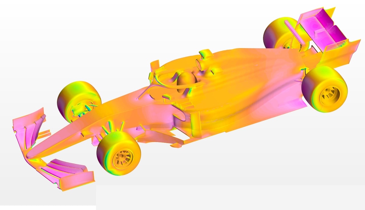
Computational Fluid Dynamics (CFD)

PINNs can be used to solve complex problems in fluid mechanics.

PINNs can incorporate the Navier-Stokes equations into their training process. These nonlinear PDEs govern fluid flow in diverse applications from aerodynamics to microfluidics. The framework enables reconstruction of complete flow fields from limited sensor data. PINNs can reveal details about turbulent structures, separation zones, and vortex dynamics.

Estimating flow fields from sparse velocity measurements is an application in which PINNs demonstrate clear advantages over traditional computational fluid mechanics methods. The physics-informed approach ensures that reconstructed fields satisfy continuity and momentum equations even in regions without direct measurements. This property makes PINNs valuable for experimental fluid mechanics, where comprehensive field measurements are challenging to obtain.

Practical cases. Try this cylinder wake demo: https://github.com/chen-yingfa/pinn-torch.

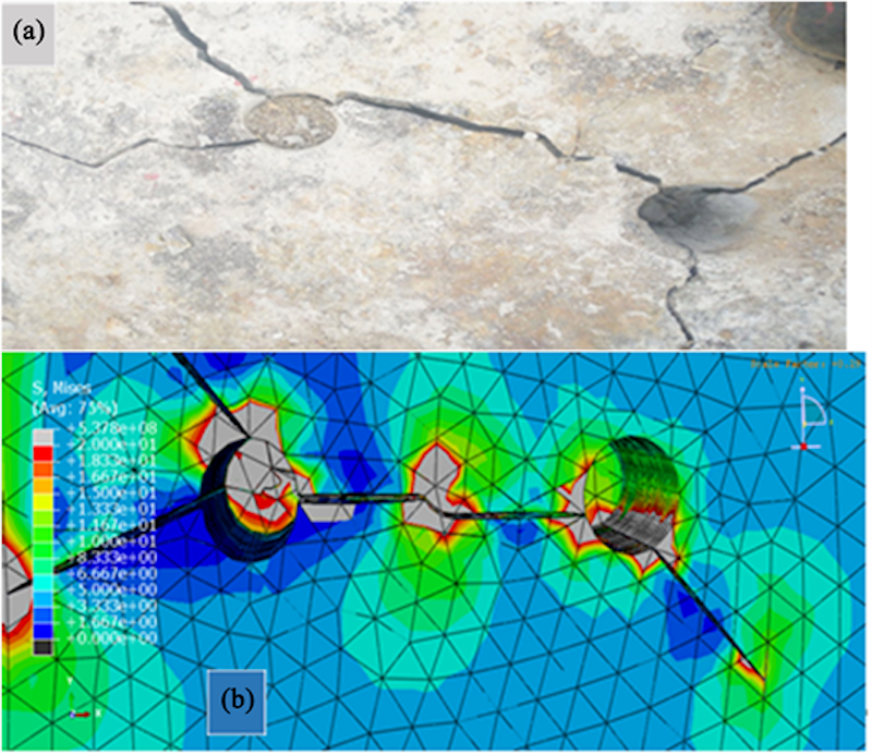
Structural Mechanics and Solid Mechanics

PINNs are used in structural systems to predict stress and strain distributions in complex structures. PINNs can solve both linear elastic behavior and nonlinear material responses; however, without the computational expense of traditional finite element analysis for every design iteration.

• Modeling material behavior, such as viscoelasticity, plasticity, and damage evolution, benefits from PINNs' flexibility. These phenomena involve complex constitutive relationships† that couple stress, strain, and internal state variables. BPINNs can capture material behavior accurately while requiring fewer experimental data points than purely empirical models.
• Simulating crack propagation in materials represents another important application where PINNs show promise. Traditional fracture mechanics approaches require adaptive meshing to track crack growth, adding significant computational complexity. The meshfree nature of PINNs allows for a more natural treatment of discontinuities and evolving damage zones. Engineers can use these models to predict failure and design more damage-tolerant structures.

Biomedical Engineering Applications

Biomedical applications present several challenges for computational modeling:

• patient-specific geometries from medical imaging
• multi-physics coupling across biological systems
• need for rapid predictions to inform clinical decisions.

In personalized models for diagnosis and treatment planning, model parameters in the PINN framework can be tuned as trainable weights to better represent patient-specific physiological features and improve simulation accuracy, as in cardiac electrophysiology.

PINNs address the above challenges by combining sparse clinical measurements with physiological principles, encoded as differential equations.

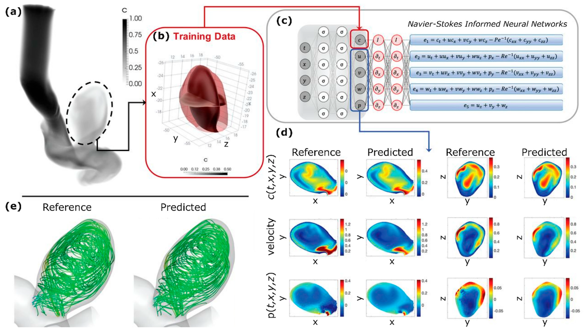
Cardiovascular Modeling and Hemodynamics

PINNs are used in biomedical engineering to simulate blood flow and cardiac mechanics, supporting the study and treatment of cardiovascular diseases.

• Modeling challenges:
  • Tortuous geometry of coronary arteries
  • Compliant, elastic vessel walls
  • Pulsatile, time-dependent blood flow
• Limitations of traditional methods:
  • Require patient-specific meshes from CT/MRI scans
  • Reconstruction can take days of expert work for a single patient
• Advantages of PINNs:
  • Embed hemodynamic principles via Navier-Stokes equations
  • Integrate patient-specific geometry directly
  • Produce personalized models for diagnosis and treatment planning efficiently

Understanding wall shear stress (WSS) and blood flow patterns is crucial for assessing cardiovascular risk. PINNs enable accurate, patient-specific modeling that combines physics with sparse clinical data:

• Wall shear stress (WSS): the force of blood on vessel walls
  • Low or oscillating WSS → correlates with atherosclerotic plaque formation
  • Extremely high WSS → may indicate aneurysm rupture risk
• Data-driven reconstruction:
  • PINNs can use sparse Doppler ultrasound or phase-contrast MRI velocity data
  • Reconstruct full 3D flow fields across the vascular tree
• Clinical advantages:
  • Assess cardiovascular risk with non-invasive imaging
  • Predict outcomes of interventions like stent placement or valve replacement
  • Evaluate how procedures alter local hemodynamics and restore healthy flow patterns

Explore a real hemodynamics PINN demo: https://github.com/alexpapados/Physics-Informed-Deep-Learning-Solid-and-Fluid-Mechanics (includes arterial blood flow cases).

Tumor Growth Modeling and Treatment Planning

PINNs can be applied in oncology to model tumor growth and predict cancer progression, providing tools for personalized treatment planning.

Tumor development represents a multi-scale, multi-physics problem.

It involves

• cancer cell proliferation,
• nutrient and oxygen transport through abnormal vasculature,
• mechanical stress from expanding cell populations,
• immune system response,
• therapeutic interventions such as chemotherapy or radiation.

Mathematical oncology has developed reaction-diffusion models that capture some of the mechanisms above, but determining parameter values for individual patients remains difficult from available clinical data.

PINNs can estimate patient-specific growth rates, diffusion coefficients, and treatment response parameters. PINNs incorporate these mechanistic models as physics constraints while simultaneously fitting to longitudinal imaging data showing tumor size and shape evolution.

Oncologists can then use these calibrated models to simulate different treatment schedules and predict which therapeutic strategy offers the best probability of tumor control for each patient.

The framework proves particularly valuable for adaptive therapy approaches, in which treatment intensity adjusts based on observed tumor response, requiring rapid model updates as new imaging data become available throughout the treatment course.

What is the Application of PINNs to Battery Technology?

PINNs can model electrochemical processes in batteries. Charge transport, chemical reactions, and thermal effects within batteries are crucial. PINNs can model these coupled physical processes. The advantage is that it requires less experimental data than traditional electrochemical models.

A battery converts chemical energy into electrical energy through electrochemical reactions, where oxidation and reduction at two electrodes move electrons through an external circuit while ions flow through the electrolyte. Inside the battery, chemical reactions and electric charge movement are tightly connected: electron flow in solid conductors is related to ion transport and reaction rates in the electrolyte and electrodes.

Battery management systems exploit models that predict state-of-charge, state-of-health, and remaining useful life. PINNs can provide these predictions while respecting the underlying electrochemical physics. The models can adapt to individual battery characteristics and aging patterns.

You may find more extensive, application-oriented discussions on battery modeling, pack design, and system optimization in the following resources:

• Battery pack design: maximizing performance and efficiency
• A guide to battery energy storage system design

What is the Application of PINNs to Semiconductors?

Engineers are leveraging high-fidelity PINN surrogate models to reduce development timelines in semiconductor manufacturing.

Problem

Semiconductor fabrication involves extremely complex, multi-step processes with tight nanometer-scale tolerances.

Some key challenges include:

• Process complexity: dozens of sequential steps (deposition, etching, lithography, implantation, annealing) where small changes cascade through the device.
• Multi-physics interactions: simultaneous chemical reactions, heat transfer, fluid dynamics, plasma effects, and mechanical stresses in materials.
• Device variability: nanoscale variations can significantly affect transistor performance, yield, and reliability.
• High cost of experimentation: each wafer run is expensive, so physical experimentation is minimized.

Solution

For example, SK hynix engineers are building AI physics surrogate models for device and process simulations (such as etch profiles) that replicate expensive Technology-CAD results at speeds up to orders of magnitude faster.

This enabled broader design exploration and faster optimization cycles.

These surrogate models approximate the behavior of high-fidelity physics simulations, running in milliseconds rather than hours, reducing development timelines while maintaining predictive accuracy.

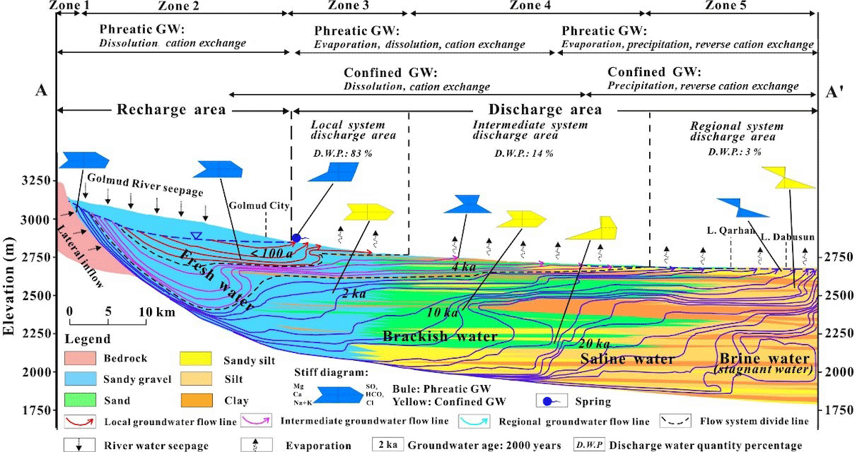
How Can PINNs Assist Geophysics and Earth Sciences?

In geophysics, PINNs help interpret seismic data to infer subsurface properties, which is crucial for oil and gas exploration.

Seismic waves propagate through the Earth according to the wave equation. Material properties determine propagation speed.

Suppose we incorporate wave physics into the learning process. PINNs can then reconstruct subsurface structure from surface measurements of seismic waves.

Examples involving solving PDEs in complex geological settings are:

• groundwater flow,
• contaminant transport,
• geothermal energy extraction.

PINNs provide a framework for incorporating both physical principles and sparse measurement data to characterize these subsurface systems. The models help engineers design remediation strategies, optimize resource extraction, and predict long-term environmental impacts.

The Emerging Role of Geometric Deep Learning

There is a consolidated approach in geometric deep learning and 3D convolutional neural networks† (3D CNNs). 3D CNNs are delivering practical solutions that designers can implement immediately.

Learn in detail about 3D CNNs.

3D CNNs approaches address the geometric nature of engineering problems. They operate directly on 3D shapes, point clouds, and mesh representations.

Learn mode on modeling meshing techniques in engineering simulations.

Here’s a summary table capturing all the key points:

Framework / Architecture

Key Idea / Domain

Strengths / Applications

Notes

Physics-Informed Neural Networks (PINNs)

Continuous function approximator constrained by PDEs

Solve problems where physics is known; requires less data

Variants can integrate with other NN architectures

3D Convolutional Neural Networks (3D CNNs)

Operate on 3D shapes, point clouds, and meshes

Rapid engineering design; pattern recognition on volumetric data; direct CAD/imaging inputs

Practical, ready-to-use in design workflows

Fourier Neural Operators (FNOs)

Frequency-space neural operator

Efficient for periodic or multi-scale problems

Ideal for problems with global interactions and spectral structure

Graph Neural Networks (GNNs)

Networks on graphs / non-Euclidean domains

Handles irregular meshes, networks, or manifold-based data

Useful for flow around complex geometries or structural analysis

Deep Operator Networks (DeepONets)

Learn mappings between function spaces

Generalizes across different input functions or boundary conditions

Can complement PINNs for parametric studies

Summary:

• PINNs leverage physics to reduce data needs and enforce consistency.
• 3D CNNs provide immediate, practical solutions for volumetric design and simulation data, and modern implementations (like Neural Concept’s) can handle irregular grids or point clouds. Learn more about the AI-first engineering platform.
• FNOs, GNNs, and DeepONets extend the neural operator framework for multi-scale, irregular, or functional problems.

3D CNNs for Design & Manufacturing

For manufacturers and design engineers, 3D CNNs and geometric deep learning offer more immediate deployment paths. These techniques can be integrated, for instance, as embedded or standalone Apps into existing design workflows.

3D CNNs can:

• Provide instant feedback on design choices
• Automate repetitive analysis tasks
• Suggest design modifications

The models learn from historical design databases and simulation results without the mathematical formulation required by PINNs.

However, combining PINNs with geometric deep learning represents an intriguing future research direction:

• PINNs provide a physics-constrained foundation for complex problems such as fluid-structure interaction (FSI).
• Geometric neural networks efficiently handle spatial complexity.

Hybrid architectures that incorporate both approaches could offer the best of both worlds: physical consistency from PINNs and geometric flexibility from specialized architectures.

Detailed Applications in Specialized Fields

PINNs address specialized technical challenges that require precise modeling of coupled physics, complex material behavior, and multi-scale phenomena. These niche applications demonstrate the framework’s adaptability to diverse physical processes.

Heat Transfer and Thermal Management

Heat transfer problems permeate engineering applications from electronics cooling to aerospace thermal protection systems. PINNs are used in various applications, including fluid mechanics, heat transfer, structural mechanics, and biomedical modeling.

Solving the heat equation with appropriate boundary conditions allows engineers to predict temperature distributions, identify hot spots, and optimize thermal management strategies.

• Thermal systems often involve coupled phenomena where heat transfer interacts with fluid flow, material deformation, or chemical reactions. PINNs handle these multi-physics problems by incorporating multiple governing equations into the loss function.
  • For example, modeling the cooling of electronics requires coupling heat conduction in solid components with convective heat transfer in cooling fluids. PINNs can solve these coupled problems without the domain decomposition and interface matching needed by traditional methods.
• Inverse heat transfer problems, where engineers must determine unknown heat sources or thermal properties from temperature measurements, benefit particularly from the PINN framework. Applications include:
  • non-destructive testing to detect defects
  • estimate heat generation in batteries
  • characterize thermal contact resistance in assemblies. The network can simultaneously solve the forward problem while estimating unknown thermal parameters.

Additive Manufacturing

PINNs enable modeling of the complex, coupled processes of additive manufacturing, enabling optimization of printing parameters and prediction of part properties without extensive experimental trials.

Additive manufacturing processes such as selective laser melting involve complex thermal, mechanical, and metallurgical phenomena that determine the final part quality. Temperature gradients during printing affect residual stress, warping, and microstructure evolution.

The layer-by-layer nature of additive manufacturing creates moving boundary conditions as material is progressively added. PINNs handle these time-dependent domains more naturally than traditional methods that require frequent remeshing. Engineers can use PINNs to design support structures, optimize scanning patterns, and predict distortion for complex geometries.

Material Processing

Material science applications benefit from PINNs’ ability to incorporate both experimental data and theoretical models of physical processes. Phase transformation kinetics, grain growth, and precipitation strengthening all follow physical laws that can be embedded into the neural network training process.

This hybrid approach enables more accurate predictions across a broader range of processing conditions than purely empirical or purely theoretical models.

Electromagnetics and Antenna Design

Electromagnetic wave propagation is governed by Maxwell’s equations, which govern electric and magnetic fields. PINNs solve these to design antennas, ensure electromagnetic compatibility, and enhance wireless systems. The vector- and coupled-nature of fields poses challenges for PINNs, which address them through their flexible framework.

Antenna design involves optimizing radiation, impedance, and bandwidth across frequencies. Traditional simulations are resource-heavy, slowing progress. PINNs trained on limited data offer quick, efficient predictions, speeding up design.

Inverse problems include determining material properties from scattering data or imaging structures using radar or medical scans. They require solving inverse-scattering problems to reconstruct material distributions. PINNs address these complex issues by integrating wave physics with measurement data.

For instance, see this article on electromagnetic RF simulation.

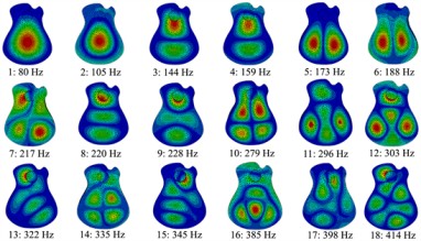
Acoustics and Vibration Analysis

Acoustic phenomena follow the wave equation, making them amenable to PINN-based modeling. Applications range from designing concert halls and reducing noise pollution to ultrasonic non-destructive testing and medical imaging. Studying how sound propagates through complex media and interacts with boundaries enables engineers to control acoustic environments and extract information from acoustic signals.

Structural vibrations represent another domain where PINNs show promise. Natural frequencies, mode shapes, and damping characteristics determine how structures respond to dynamic loads. PINNs can model these systems while incorporating boundary conditions and material properties. Engineers use these models for vibration-isolation design, fatigue-life prediction, and structural health monitoring.

Modal analysis traditionally requires solving eigenvalue problems† derived from discretized structural models. PINNs offer an alternative approach where modes emerge naturally from training on vibrational data. This data-driven approach can identify modes even when the structural model is uncertain or when nonlinear effects complicate traditional linear modal analysis.

Learn more about structural vibration, which includes an educational explanation of eigenvalue problems.

Challenges and Limitations of Physics-Informed Neural Networks

PINNs still face obstacles that currently limit their widespread adoption in production engineering environments. In this section, we will discuss when PINNs are a good solution and when alternative approaches may be more appropriate.

Computational Training Costs

Despite their advantages, PINNs face several challenges that limit their adoption in true production engineering environments.

Training PINNs can be computationally expensive, especially for large and complex problems. The network must undergo a process that requires many iterations to converge. This is particularly true for problems with multiple scales or stiff dynamics:

• evaluate the loss function at numerous collocation points,
• compute derivatives through automatic differentiation,
• update potentially millions of parameters.

The computational cost depends on the problem dimensionality, the complexity of the equations, and the desired accuracy. Three-dimensional problems with time dependence require evaluating the network over a four-dimensional space, which imposes substantial memory and computational requirements. Hardware acceleration with GPUs partially mitigates these costs, but training times for complex problems can still run for hours or even days.

Optimization challenges arise from the non-convex nature of neural network training.

The loss landscape contains numerous local minima, and the network may converge to solutions that satisfy the data but violate physics, or vice versa. Balancing the different loss terms requires careful tuning, and optimal weighting strategies remain an active area of research. Adaptive weighting schemes that adjust term importance during training show promise but introduce an additional layer of complexity.

Handling Discontinuities and Multiscale Problems

Three fundamental challenges limit PINNs in certain problem classes:

1. representing sharp discontinuities,
2. capturing phenomena across vastly different scales, and
3. predicting chaotic systems with sensitive dependence on initial conditions.

Discontinuities and Sharp Transitions

PINNs can struggle with highly discontinuous complex systems, such as shock waves or chaotic flows. Neural networks are inherently biased toward smooth functions because standard activation functions produce continuous outputs.

• For instance, when a shock wave in supersonic flow creates a near-instantaneous jump in pressure, density, and velocity, the network must use steep gradients and many parameters to approximate this discontinuity. The physics loss computed near the discontinuity produces large residuals that dominate training, yet the network architecture fundamentally resists representing the sharp transition.
• Contact discontinuities in multiphase flows present similar difficulties. Oil and water flowing together create a material discontinuity where density and viscosity change abruptly, even though velocity and pressure remain continuous.
• Fracture mechanics introduces discontinuities where displacement fields are continuous, but their spatial derivatives jump across crack surfaces.

Specialized techniques include adaptive activation functions that adjust their shape during training, domain-decomposition methods that train separate networks on either side of discontinuities, and extended physics-informed neural networks that incorporate enrichment functions to explicitly represent discontinuous features.

Multiscale Phenomena

• Turbulent flows contain eddy structures ranging from meters in an aircraft wake down to millimeters at the Kolmogorov microscale†. A network trained to capture large-scale patterns may miss small-scale features, whereas a network that represents the smallest scales becomes prohibitively expensive to train.
• Battery dynamics couple electrochemical reactions occurring on the microsecond timescale with thermal evolution unfolding over hours, spanning eight orders of magnitude. Training a single network across such disparate scales strains both representational capacity and numerical conditioning.
• Sequential multiscale strategies train separate networks for different scale ranges and couple them through interface conditions. Hierarchical architectures specialize different layers for different scales. Fourier neural operators decompose solutions into frequency components, providing better multiscale handling than standard feedforward networks.

Can Neural Networks Model Chaotic Dynamical Systems?

Neural Networks can model chaotic systems accurately, but they require careful attention because chaos can amplify errors, and learning might introduce new instabilities.

Chaotic systems are very sensitive to initial conditions, meaning tiny errors can cause their trajectories to diverge rapidly.

While classical methods face similar challenges, neural networks can sometimes amplify errors unpredictably during training. Even if a model aligns well with physics on training data, it might still exhibit unwanted instabilities or develop artificial attractors when tested with unseen starting points. Additionally, the nonconvex nature of optimization landscapes means different training runs can converge to different local minima, leading to varied out-of-sample results.

That’s why using ensemble approaches (training multiple networks) and examining prediction variance are so helpful to understand the uncertainty involved.

Learn more about uncertainty quantification.

Data Quality and Availability

PINNs generally require less data than purely data-driven machine learning models.

However, data quality still strongly affects performance:

• Noisy or sparse measurements can make training difficult, especially when the physics loss and data loss conflict. The network may ignore physics to fit noisy data, or ignore data to satisfy physics, depending on the loss weighting. Developing robust strategies that account for measurement uncertainty is an ongoing challenge.
• The spatial and temporal distribution of training data is also critical. Data collected only at boundaries provides limited information about the internal states. Sparse temporal measurements make it harder for the network to learn dynamics. Optimal experimental design is still underexplored. Active learning approaches iteratively select new measurement points. They show promise in addressing this issue.
• Systematic errors or biases in measurement data pose additional challenges. The network can reproduce these biases while still approximately satisfying the governing equations. Validation with independent data and simple physical reasoning is essential.

Generalization and Transfer Learning

A trained PINN typically solves one specific problem with fixed geometry, boundary conditions, and parameters. Applying the trained network across different conditions requires retraining, which limits the efficiency gains.

Recent architectures like DeepONets† and Fourier neural operators† address this limitation. Learning operators map between function spaces, enabling generalization across different input conditions. However, these approaches add complexity. They may sacrifice some of the physical guarantees of standard PINNs.

Transfer learning, in which a network trained on one problem serves as a starting point for related problems, offers another path toward more efficient training. The network can learn general representations of physics that transfer across similar applications, reducing training time for new cases. However, effective transfer learning strategies for PINNs remain less developed than other areas of deep learning.

See an example of various techniques, including the transfer learning process.

Use Cases

PINNs are transitioning from academic curiosity to practical industrial deployment. This chapter documents real-world applications in which PINNs have solved engineering problems, achieving computational speedups ranging from 100× to 1,000,000× compared to conventional methods. Each use case presented here includes verified implementations with documented technical architectures, data sources, and quantifiable performance metrics.

The listed industrial applications demonstrate that PINNs have evolved beyond proof-of-concept to become production-ready tools for specific problem classes. The most successful deployments share common characteristics: well-defined physics, sparse measurements, the need for real-time inference, or the need for expensive conventional simulations.

Challenges remain, particularly for complex 3D geometries.

Learn more about the AI Design Copilot by Neural Concept, a ground-breaking platform for engineering teams.

Organization (Year)

Application

Speedup

Source

SoftServe + NVIDIA (2024) -see how predictive AI models based on 3D deep learning leverage CAD and CAE data.

Virtual flow metering for ESP oil wells - real-time flow rate estimation

Not quantified

Exploring the potential of PINNs

Global Oil & Gas + SoftServe (2024)

Fischer-Tropsch reactor optimization - microkinetics modeling

10⁶× (1 million)

Exploring the potential of PINNs

Ansys + NVIDIA (2021)

Power electronics thermal management - heat transfer analysis for semiconductors

Not quantified

PINNs for Heat Transfer

Ansys + NVIDIA Modulus (2024)

Semiconductor design - multi-physics simulation for GPUs, HPC chips

100× (for thermal simulations)

NVIDIA Developer

Purdue University (2022)

Nuclear reactor monitoring - digital twin for PUR-1 reactor start-up

Real-time capable

PINN Solution of Point Kinetics Equations for a Nuclear Reactor Digital Twin

Chung-Ang University (2024)

Spacecraft trajectory optimization - minimal-thrust swingby paths

30× fewer iterations

Nature

NVIDIA (2024)

Oil reservoir characterization - Norne field history matching using PINO

100-6000×

https://arxiv.org/abs/2406.00889

Siemens Energy (2024)

Turbomachinery aerodynamic design - gas turbine and compressor analysis

10,000×

NVIDIA Blog

University of Cagliari (2025)

NH₃ oxidation plug flow reactor - inverse parameter estimation

Not quantified

ACS Industrial & Engineering Chemistry Research

DLR (German Aerospace Center)(2025)

Transonic airfoil flows - 2D Euler equations with artificial viscosity for shock wave stabilization

100,000×

PINNs for inviscid transonic flows around an airfoil

Summary by Sector

Sector

Speedup Range

Primary Application

Technology Maturity

Oil & Gas

100-6000×

Flow metering, reservoir simulation

Production deployment

Chemical Processing

10⁶×

Reactor optimization

Pilot/Production

Power Electronics

N/A

Thermal design

Commercial tools

Semiconductors

N/A

Multi-physics simulation

Commercial integration

Nuclear

Real-time

Reactor monitoring

Research/Pilot

Aerospace

30× fewer iterations

Trajectory optimization

Research

Turbomachinery

N/A

Aerodynamic design

Production deployment

Summary - Key Observations

• Most dramatic speedups (100- to 1,000,000×) occur in iterative inverse problems and parametric studies.
• Hybrid PINN approaches (combining physics with data) outperform pure physics or pure data methods.
• Commercial adoption is highest in sectors with mature digital infrastructure (energy, semiconductor, aerospace).
• Real-time monitoring applications benefit from fast PINN inference even when training is expensive.

Summary - Technical Patterns

• Network architectures: 4-8 hidden layers, 20-50 neurons per layer are common
• Optimizers: Adam (initial training) + L-BFGS (fine-tuning) is standard practice
• Loss functions: Weighted sum of data loss + PDE residuals + boundary/initial conditions
• Hardware: NVIDIA GPUs (A100, H100) standard for training; inference often CPU-capable
• Frameworks: NVIDIA Modulus, DeepXDE, most commonly cited

Future Directions and Research Frontiers

The field of physics-informed neural networks continues evolving rapidly as researchers address current limitations and explore new capabilities. These developments promise to expand the applicability of PINNs. Also, interdisciplinary collaborations are essential for advancing PINNs, combining expertise from physics, engineering, and machine learning.

Algorithmic Improvements

Future directions for PINNs include advancements in algorithmic techniques to improve efficiency and scalability. Researchers are developing adaptive training strategies that automatically adjust the distribution of collocation points, the weighting of loss terms, and the network architecture during training. These meta-learning approaches aim to reduce the manual tuning currently required for successful PINN applications.

• Multi-fidelity approaches that combine low-cost approximate models with expensive high-fidelity data represent another promising direction. The network can learn from abundant low-fidelity simulations while correcting biases using limited high-fidelity measurements. This strategy leverages the strengths of both data sources to improve prediction accuracy and reduce experimental costs.
• Ensemble methods that train multiple PINNs with different initializations or architectures provide estimates of prediction uncertainty. Variance across ensemble members indicates regions where the model is less confident, helping engineers identify where additional data or analysis is needed. Bayesian approaches to PINN training offer an alternative framework for uncertainty quantification.

Large-Scale and Real-Time Applications

Large-scale and real-time applications of PINNs require improvements in scalability, efficiency, and deployment. Reducing training time through better optimization algorithms, parallel computing strategies, and hardware acceleration remains critical. Once trained, PINNs can provide rapid predictions, but deploying these models in embedded systems or edge computing environments requires further work on model compression and efficient inference.

• Digital twins maintain a current model of a physical asset by continuously assimilating sensor data and updating predictions. PINNs naturally support this approach by solving inverse problems and assimilating sparse measurements. Applications include monitoring infrastructure health, optimizing manufacturing processes, and predicting equipment failures.
• The integration of PINNs with control systems enables physics-informed reinforcement learning for autonomous systems. The PINN provides a differentiable model of system dynamics, allowing gradient-based optimization of control policies that respect physical constraints. Applications span robotics, autonomous vehicles, and process control.

Integration with Traditional Methods

Hybrid approaches combine PINNs with traditional numerical methods, leveraging the strengths of each; the two methods can be coupled through interface conditions that ensure continuity of solutions and fluxes:

• Finite element analysis provides accurate solutions in regions with complex geometry or material properties
• PINNs handle regions where measurements are available but governing equations may be uncertain.

Data assimilation frameworks that incorporate PINN-based models offer new opportunities to combine simulation and measurement. As new experimental input data becomes available, the PINN can be retrained to incorporate this information, improving predictions. Sequential data assimilation for time-dependent problems allows the model to track evolving conditions.

Reduced-order modeling (ROM) represents another area where PINNs and traditional methods complement each other. Traditional projection-based reduced-order models provide computational efficiency but may sacrifice accuracy. PINNs can learn reduced representations that capture essential physics while maintaining physical consistency through the physics-informed loss terms.

Getting Started with PINNs: Practical Checklist

Follow these steps to quickly set up a PINN, from defining the problem to deploying predictions.

Here’s an ultra-compact checklist you can follow:

Step n°

Action

Note

1

Problem

PDEs, BC/IC

2

Data

Training & validation

3

Network

Layers, neurons, activation

4

Loss

Data + PDE + BC/IC

5

Train

Optimizer, LR, stopping

6

Debug

Gradients, small test

7

Validate

Compare to data/analytics

8

Deploy

Predictions, surrogate

Conclusions

Physics-informed neural networks have matured into a powerful hybrid paradigm, merging the data-driven flexibility of deep learning with the reliability of physical laws encoded in differential equations. PINNs enable engineers to solve forward and inverse problems with remarkable data efficiency, continuous differentiable solutions, and native handling of complex geometries. Those benefits become evident in areas where experimental data is limited or costly.

Real-world deployments already demonstrate dramatic speedups: from 10,000× reductions in simulation time at ExxonMobil and Siemens to rapid patient-specific hemodynamics models in clinical settings. These gains stem from PINNs’ ability to act as accurate surrogates while respecting conservation principles.

Nevertheless, significant hurdles remain that prevent broader industrial adoption:

• Scalability to large 3D transient problems: Training costs often explode due to the need for millions of collocation points and stiff loss landscapes, limiting routine use on full-scale engineering models
• Robust handling of discontinuities and multiscale physics: Standard architectures struggle with shocks, interfaces, or phenomena spanning orders of magnitude in length/time (e.g., turbulence, fracture, battery micro-macro coupling)
• Transferability and generalization: Most PINNs are tailored to specific geometries/parameters; zero-shot application to new configurations often degrades performance.
• Optimization pathologies: Competing gradients between data-fitting and physics-enforcement terms often lead to stagnation or convergence to poor local minima, necessitating extensive hyperparameter tuning.

Recent advances like Ψ-NN (2025), which automatically discovers and hard-wires physical structures (symmetries, invariances) into the architecture itself, directly address generalization and training stability, pointing toward more autonomous and reliable physics-informed models.

Looking ahead, the most impactful engineering workflows will intelligently blend PINNs with traditional solvers, operator learning (FNOs, DeepONets), and geometric deep learning.

This multi-method ecosystem promises to accelerate design cycles while preserving the trustworthiness demanded by safety-critical applications.

FAQ

Can PINNs beat FEM?

PINNs and FEM serve different purposes. FEM offers validated tools with convergence guarantees for known equations and complex geometries. PINNs are advantageous when data are available, but equations are uncertain, for inverse problems, or for rapid iterations without remeshing. Often, combining both approaches strategically benefits engineering practice.

What is the difference between physics-informed neural networks and traditional neural networks?

Traditional neural networks learn only from data, often needing large datasets and risking unrealistic predictions when extrapolating. PINNs incorporate physical laws into the loss function, enabling learning with less data while respecting principles such as conservation of mass and energy.

What are the main applications of physics-informed neural networks?

PINNs are applicable across diverse engineering domains, including fluid dynamics, structural mechanics, heat transfer, biomedical modeling, materials science, and geophysics.

What are the key limitations of physics-informed neural networks?

Key limitations include high training costs for large 3D problems, difficulty in modeling sharp discontinuities such as shock waves, challenges with multiscale systems, sensitivity to hyperparameters, limited generalization beyond the training data, reliance on well-formulated physics-informed loss functions, and the need for high-quality data.

Which are the best Python libraries for building physics-informed neural networks?

DeepXDE provides a high-level PINN interface that supports governing equations and boundary conditions. PyTorch and TensorFlow provide detailed control with automatic differentiation. JAX focuses on composable functions and efficiency. SciANN simplifies PINN setup through intuitive tasks. NeuralPDE connects with Julia’s ecosystem.

How are physics-informed neural networks used in fluid dynamics?

In fluid dynamics, PINNs embed the Navier-Stokes equations during training to ensure that velocity and pressure fields satisfy conservation laws. Usage covers aerodynamics, microfluidics, multiphase flows, and turbulence, where traditional CFD is costly.

What Is Ψ-NN?

Ψ-NN (Physics Structure-Informed Neural Network, 2025) is an advanced PINN variant that automatically discovers and embeds physical structures directly into the network architecture, e.g., symmetries, conservation laws. Ψ-NN uses a 3-step process: train a teacher PINN, extract parameter relations (e.g., weight symmetries), and reconstruct a studentnetwork with hard-wired physics.

How Can I Implement Ψ-NN?

Code Implementation is available on GitHub at https://github.com/ZitiLiu/Psi-NN (archived on Zenodo: https://doi.org/10.5281/zenodo.17098398).

Bibliography

• Cai, S., Mao, Z., Wang, Z., Yin, M., & Karniadakis, G. E. (2021). Physics-informed neural networks (PINNs) for fluid mechanics: A review. Acta Mechanica Sinica, 37(12), 1727-1738.
• Cuomo, S., Di Cola, V. S., Giampaolo, F., Rozza, G., Raissi, M., & Piccialli, F. (2022). Scientific machine learning through physics-informed neural networks: Where we are and what’s next. Journal of Scientific Computing, 92(3), 88.
• Haghighat, E., Raissi, M., Moure, A., Gomez, H., & Juanes, R. (2021). A physics-informed deep learning framework for inversion and surrogate modeling in solid mechanics. Computer Methods in Applied Mechanics and Engineering, 379, 113741. Mao, Z., Jagtap, A. D., & Karniadakis, G. E. (2020). Physics-informed neural networks for high-speed flows. Computer Methods in Applied Mechanics and Engineering, 360, 112789.
• Karniadakis, G. E., Kevrekidis, I. G., Lu, L., Perdikaris, P., Wang, S., & Yang, L. (2021). Physics-informed machine learning. Nature Reviews Physics, 3(6), 422-440.
• Kissas, G., Yang, Y., Hwuang, E., Witschey, W. R., Detre, J. A., & Perdikaris, P. (2020). Machine learning in cardiovascular flows modeling: Predicting arterial blood pressure from non-invasive 4D flow MRI data using physics-informed neural networks. Computer Methods in Applied Mechanics and Engineering, 358, 112623.
• Liu, Z., Liu, Y., Yan, X. et al. Automatic network structure discovery of physics informed neural networks via knowledge distillation. Nat Commun 16, 9558 (2025
• Lu, L., Meng, X., Mao, Z., & Karniadakis, G. E. (2021). DeepXDE: A deep learning library for solving differential equations. SIAM Review, 63(1), 208-228.
• Raissi, M., Perdikaris, P., & Karniadakis, G. E. (2019). Physics-informed neural networks: A deep learning framework for solving forward and inverse problems involving nonlinear partial differential equations. Journal of Computational Physics, 378, 686-707.
• Sahli Costabal, F., Yang, Y., Perdikaris, P., Hurtado, D. E., & Kuhl, E. (2020). Physics-informed neural networks for cardiac activation mapping. Frontiers in Physics, 8, 42.
• Wang, S., Teng, Y., & Perdikaris, P. (2021). Understanding and mitigating gradient flow pathologies in physics-informed neural networks. SIAM Journal on Scientific Computing, 43(5), A3055-A3081.

† Technical Vocabulary

• 3D convolutional neural networks (3D CNNs): Neural networks that process volumetric data (CAD models, medical scans) by applying filters with weights w across three spatial coordinates (ijk) in an input volume x: yᵢⱼₖ = σ(∑∑∑ wₐᵦᵧ · xᵢ₊ₐ,ⱼ₊ᵦ,ₖ₊ᵧ + b). Unlike 2D CNNs (images), 3D CNNs capture spatial relationships in all three dimensions simultaneously, which is helpful for volumetric shapes.
• Activation function: A nonlinear map σ that transforms a neuron’s pre-activation z = w·x + b into an output a = σ(z), enabling networks to represent non-linear functions.
• Adam (Adaptive moment estimation): a widely used optimizer for training neural networks that adjusts the learning rate individually for each parameter. With Adam, training is faster and more reliable. The optimizer adaptively adjusts a global learning rate α per model parameter θ using momentum and gradient variance, e.g., mₜ = β₁mₜ₋₁ + (1 - β₁)gₜ (momentum), vₜ = β₂vₜ₋₁ + (1 - β₂)gₜ² (variance), θₜ₊₁ = θₜ - α·mₜ/√vₜ (update). Typical values are α=0.001, β₁=0.9, β₂=0.999. Note that each parameter gets its own effective learning rate through the mₜ/√vₜ scaling.
• Constitutive relationships: Mathematical equations that describe material behavior, such as how stress relates to strain in a specific material. For instance, the σ=σ(ε) relationship (stress vs. strain) could be σ = E ε (Hooke’s law: linear elastic) or σ = σ₀ + K εⁿ (power-law hardening), etc.
• DeepONets: Deep Operator Networks; architectures that learn mappings between function spaces rather than point-wise predictions.
• Differentiable: A function whose derivative exists at every point, allowing calculation of rates of change.
• Discretization: Process of dividing a continuous domain into discrete elements (mesh, grid) for numerical computation. Continuous functions f(x) are converted into discrete values fᵢ = f(xᵢ), enabling numerical solution of differential equations.
• Eigenvalue: Scalar value associated with a system that characterizes specific modes of behavior (e.g., natural frequencies in vibration). In math: [K - ω²M] φ = 0 gives natural frequencies ωₙ (eigenvalues) and mode shapes φₙ(eigenvectors) of a vibrating structure, where K is the stiffness matrix, and M is the mass matrix.
• Fourier Neural Operators (FNOs): Neural operators that learn mappings between function spaces by evolving solutions in frequency space. FNOs efficiently capture global, multi-scale structure and remain resolution-independent.
• Hessian: Matrix of 2nd-order partial derivatives; describes curvature of the loss landscape in optimization.
• Kolmogorov microscale: The shortest length scale in turbulent flow where viscous dissipation dominates, revealing the hidden fluid mechanics beneath chaotic motion. At this scale, inertial effects vanish, velocity gradients smooth out, and kinetic energy is irreversibly converted into heat. It marks the endpoint of the turbulent energy cascade and defines the minimum scale required to resolve turbulence accurately.
• L-BFGS: Limited-memory Broyden-Fletcher-Goldfarb-Shanno algorithm; a 2nd-order optimization method approximating the Hessian.
• Learning rate scheduling: a training technique that adjusts the learning rate during training, typically decreasing it over time to allow larger steps early to accelerate progress and smaller steps later to ensure precise convergence.
• Schroedinger equation: the fundamental equation of quantum mechanics that describes how the quantum state (wave function ψ) of a physical system evolves.
• Universal approximation theorem: A theorem stating that neural networks can approximate any continuous function given sufficient width.
• Viscoelasticity: A material property exhibiting both viscous (fluid-like) and elastic (solid-like) behavior under deformation.
• Vorticity: Measure of local rotation in a fluid flow field; the curl of the velocity vector.
• Xavier or He initialization: Xavier (Glorot) initialization uses variance 1/n (n = average of input/output units) to keep activation variance stable across layers, suited for tanh/sigmoid. He (Kaiming) initialization uses variance 2/n(n = input units) for ReLU variants to compensate for rectification and avoid vanishing gradients in deep networks.

‍