Computational Fluid Analysis - Applications and Benefits

Computational fluid dynamics (CFD) is a powerful tool for engineers. CFD software enables engineers to understand how fluids behave and how heat is transferred in a virtual environment.

Today’s engineers need to know CFD. Companies invest in CFD because it predicts fluid behavior and heat transfer before prototypes are built, enabling product improvements early in the design process.

In industry, CFD is most effective when integrated with design tools such as CAD. This combination allows engineers to iterate on geometry and operating conditions, progressively refining performance. CFD is widely used to optimize designs for improved performance, such as enhancing efficiency and reducing fuel consumption across industries like aerospace and automotive.

We provide an introduction to CFD, explain its main ideas, demonstrate its use, identify its limitations, and discuss how it fits into real design workflows.

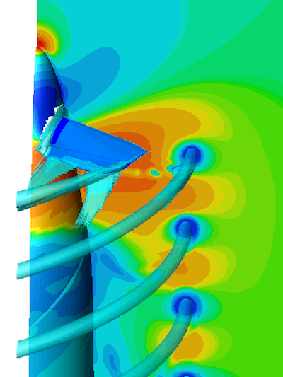
Beyond saving money, CFD solves complex problems across fields such as automotive and aerospace. CFD is used to simulate and analyze problems that involve fluid flows, such as aerodynamic and aeroacoustic phenomena.

• In aerospace product design, engineers use CFD to predict aerodynamic forces and aeroacoustic phenomena, such as noise generated by aircraft engines and landing gear, supporting both performance optimization and noise-reduction strategies.
• Imagine also space applications:
• aerodynamic heating during spacecraft re-entry;
• air recirculation, thermal control, and comfort in enclosed environments such as space stations, or the thermal design of satellites.
• In the automotive industry, for example, CFD is used to optimize vehicle aerodynamic design by simulating airflow over car bodies, thereby reducing drag and improving fuel efficiency. Explore the CAE and CFD tools used in the automotive industry.
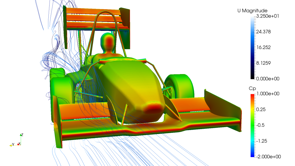
• Imagine also Formula One applications:
• fine-tuning the aerodynamic performance of an F1 car (see more details on Formula 1 aerodynamics);
• optimizing engine performance (internal flows, heat transfer, and chemical reactions).

CFD is particularly valuable for analyzing complex geometries. Think of intricate shapes and moving boundaries in an engine that are challenging to study experimentally.

Here is a concise journey in this fascinating and highly visual discipline.

• Fluid Dynamics and Heat Transfer - Introduction
• CFD vs. Physical Testing Cycle
• CFD Solution - Workflow
• CFD - History and Status
• Algorithms
• What Are the Key Applications of CFD Analysis?
• CFD - Advanced
• Challenges and Limitations of CFD
• Best Practices for CFD
• CFD In a Nutshell - Final Summary
• Future of CFD
• FAQ
• APPENDIX 1: The Lattice Boltzmann Method
• APPENDIX 2: Finite Volumes - A Look “Under the Hood”

Fluid Dynamics and Heat Transfer - Introduction

Fluid dynamics studies how fluids accelerate, decelerate, or change direction in response to applied forces. Properties like density, viscosity, and compressibility shape fluid behavior. Heat transfer accompanies many flows, with convection carrying energy via bulk motion, conduction through molecular collisions, and radiation, which is less dominant in most engineering cases.

Analytical Solution

Analytical solutions exist only for simplified cases, so numerical methods prove essential for realistic geometries and conditions. Governing equations enforce conservation principles.

• The continuity equation maintains mass balance: ∇·(ρu) = 0 for incompressible flows, with adjustments for density variations otherwise.
• The momentum equation balances acceleration due to pressure, viscous forces, and external forces. The energy equation accounts for thermal effects, including work and heat addition.

Turbulence

Turbulence emerges when flow becomes disordered (see figure). Turbulence is not negative in absolute terms. It combines momentum, heat, and species far more efficiently than laminar diffusion: in other words, it’s a boost for transfer efficiency. However, it increases drag. For sure, it complicates prediction due to its vast range of interacting scales.

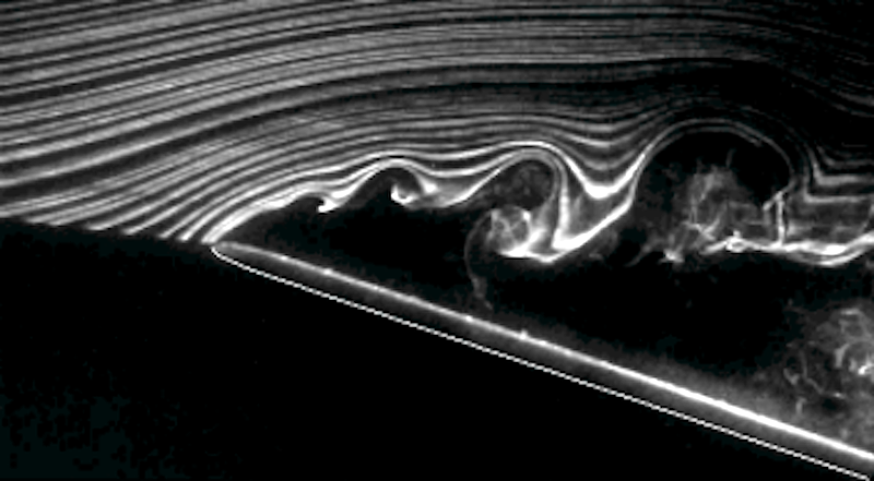
When inertial forces exceed viscous damping, the flow loses stability. Perturbations grow, forming vortical structures that break down through a cascade to smaller scales.

Energy transfers from the large-scale mean flow to progressively smaller eddies, similar to how a large object shattering produces fragments of various sizes. This process cascades through intermediate scales (the inertial range) until it reaches the smallest turbulent structures, known as the Kolmogorov scale η, where viscosity dissipates the energy as heat. Most CFD approaches do not resolve phenomena at this tiny scale; only Direct Numerical Simulation (DNS) can explicitly capture all eddy sizes down to the Kolmogorov scale, η.

The Navier-Stokes Equations and Energy Transport (Incompressible Case)

The fundamental basis of almost all CFD problems is the Navier–Stokes equations, which describe the motion of fluid substances.

• Since flow occurs in 3D space, students encounter vector notation.
• The main symbols are velocity field u, pressure p, density ρ, and viscosity μ.
• It is also important to consider spatial change using the gradient notation ∇.

Momentum Transport (Navier-Stokes equations)

The momentum equation balances inertia, pressure forces, viscosity, and external forces.

In incompressible form, it reads:

ρ (∂u/∂t + u·∇u) = -∇p + μ ∇²u + f

Here,

• ∂u/∂t captures time-dependent (unsteady) phenomena,
• u·∇u is the highly nonlinear convection term,
• -∇p is the pressure gradient driving flow,
• μ ∇²u is viscous diffusion, and
• f represents body forces like gravity.

With continuity:

∇·u = 0

Energy Transport

Note that energy transfer enters through an additional law, not implicitly through Navier–Stokes, with additional variables such as .cₚ, T, Φ, and Q:

ρ cₚ (∂T/∂t + u·∇T) = k ∇²T + Φ + Q

This equation couples to Navier-Stokes, in fact:

• Velocity u from the Navier–Stokes equations drives convective heat transport; without it, CFD can solve conductive heat transport.
• Temperature T affects material properties (μ, ρ, k, cₚ)
• In buoyant flows, temperature T feeds back into momentum via body forces (e.g, the Boussinesq term)

CFD vs. Physical Testing Cycle

Consider the traditional way to check a car’s or airplane’s aerodynamic performance. Engineers placed a full physical sample or a scaled model in a fluid volume, the wind tunnel (see figure). Engineers measured, for instance, drag and lift with balances and sensors. To visualize flow patterns, they used smoke streams or surface tufts to show separation, vortices, and attachment points.

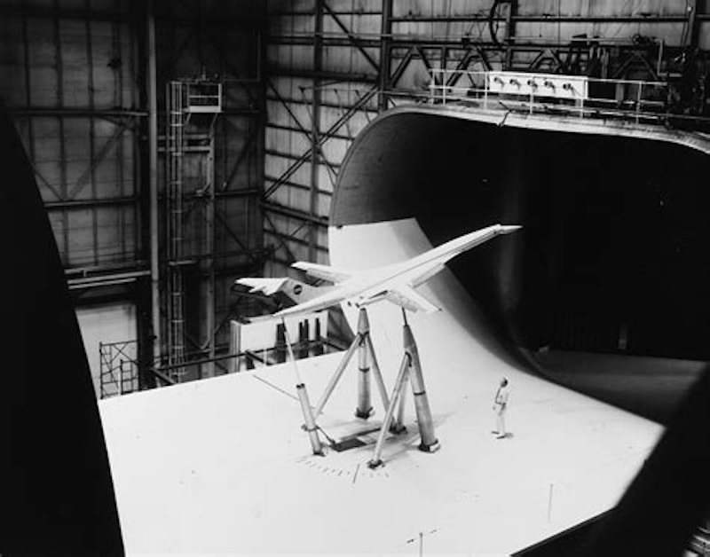
Managing a full automotive or aerospace wind tunnel is very costly and time-consuming. It requires high-energy fans, precise climate control, belts that match road speed, and careful setup to avoid errors caused by walls or models.

Tests can only be conducted on physical objects, and this slows the testing process. What type of object?

• Testing production cars or airplanes would yield results only after it is too late to influence design.
• Engineers need to deliver early aerodynamic data from prototypes, such as clay or fiberglass models. However, these need new parts and tunnel time for every change.

Smoke offers visual clues about surface flow. However, it is limited, showing only near-body patterns and missing deep-wake structures. It provides no quantitative data on pressure, internal flow, or unsteady motion (additional tools are needed).

In summary, the traditional physical testing cycle presents several key drawbacks, including high costs, long lead times, and limited insight. The following section provides a structured comparison of these limitations with the advantages of computational fluid dynamics (CFD).

Drawbacks of the Traditional Testing Cycle

The constraints of a wind tunnel highlight three fundamental drawbacks of the physical testing cycle in general:

1. High Cost: Prototypes use materials, labor, and machining time. Even if testing is outsourced, testing sessions are billed at high hourly rates. Prototype building and changes add more expense. CFD sharply reduces these costs by reducing physical builds and testing hours.
2. Long Lead Times: Prototyping, booking testing slots, and re-testing slow everything down. One small change can delay the project by days or weeks. CFD runs many versions in the time it takes one physical test.
3. Limited Insight: Experimental data, such as from a wind tunnel, provide overall forces and some surface pressures, but coverage remains limited. Smoke or tufts show only surface views and cannot easily reveal full three-dimensional flow or turbulence details.

CFD Solution - Workflow

Computational Fluid Dynamics (CFD) solves the problems highlighted in the previous section.

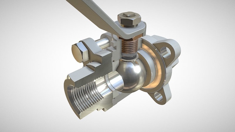
CAD

Engineers work with digital CAD models from the start. Surfaces defined by CAD act as boundaries for the fluid domain. The big trouble is that CAD files are normally built to describe the solid rather than the fluid domain (as illustrated).

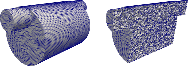
Meshing, Physics, Boundary Conditions

After geometry modelling in CAD software, engineers build a computational mesh, select appropriate physics models, and set boundary conditions, such as the inlet velocity. The “mesher” is a key component of analysis software. Nowadays, in most cases, meshing is fully integrated into the CFD platform. Meshing must often accommodate complex geometries, including intricate shapes or moving parts, to ensure accurate simulation results.

Solver

Using powerful HPC (High Performance Computing) resources, either locally or in the cloud, engineers use software that solves the governing equations for momentum, mass, and energy transport via numerical analysis. The numerical process is quite slow (hours to days), especially on a few processors.

Postprocessing

Results of the CFD analysis include fluid mechanics quantities of interest, such as velocity, pressure contours, and streamlines. Also, overall or local key parameters, such as surface force coefficients.

Apply CFD to Design

Virtual (computational) models reduce experimental costs by enabling virtual investigation of multiple design configurations. CFD facilitates design modifications, such as adjustments to spoilers or mirrors, and provides results within hours rather than weeks. Once validated, modern CFD tools yield results that closely correspond to wind-tunnel data.

In engineering practice, CFD and physical testing serve complementary roles.

CFD is used for early exploration and optimization to identify strong concepts, while wind tunnel testing validates the final design under controlled conditions.

This integrated approach speeds up development, reduces risk, and controls costs.

Need for Speed: Cloud Computing and Machine Learning

CFD simulations can be costly and time-consuming, often requiring hours to days of computation on a single workstation for complex problems.

For example, simulating turbulent flow around an automobile may require hundreds of gigabytes of memory and several days of runtime on a single processor.

• To address this, CFD uses parallel computing, distributing calculations across multiple processors to reduce computational time. Ideally, scaling is linear, but actual gains diminish due to communication overhead. Large-scale simulations often use hundreds or thousands of processors to achieve practical turnaround times.
• Given the amount of investment in hardware, IT capabilities, and energy consumption, many companies access HPC via Cloud Computing.
• New methods reduce hardware, management, and energy costs. AI tools, especially machine learning and deep learning, provide real-time feedback during design, enabling quick iterations and optimizations. Machine learning (see next chapter) integrates with computational fluid dynamics to overcome traditional limitations in speed and complexity.

How Can Machine Learning and CFD Integrate?

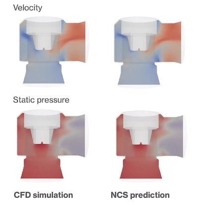
CFD produces large amounts of high-fidelity data. Machine learning uses this data to learn mappings between inputs and outputs, creating predictors or surrogates of CFD solvers.

These faster approaches offer speed gains of several orders of magnitude.

Deep learning adapts computer vision techniques to learn mappings from CAD geometry into CFD-relevant representations such as pressure or temperature fields.

Neural Concept and CFD

Neural Concept’s platform uses 3D deep learning to “understand” CAD geometries. It learns their interactions with physics. Learning feeds on CFD result data.

Neural Concept employs geodesic convolutional neural networks (3D CNNs). 3DCNNs operate directly on shapes. They predict velocity and pressure distributions, as well as performance metrics. The advantage is having the prediction in milliseconds rather than hours.

Simply explained, a 3D CNN works like this:

Physics output = Activation of ( Σ Shape features × Learned filters )

Meaning:

• The shape is decomposed into local geometric features.
• learned filters detect patterns linked to flow behavior
• Combining them produces instant physics predictions.

Instant physics predictions are possible because the computational unit of a neural network is just a weighted sum followed by a nonlinear activation.

y = σ( w · x + b )

Once trained, inference is only made of multiply-add operations! This accelerates design cycles dramatically.

• For example, partnerships with Orbital Stack reduced wind-simulation iteration times from 10 hours to minutes by leveraging vast urban wind datasets.
• In automotive and aerospace, neural predictors enable thousands of design iterations per day for external aerodynamics, heat exchangers, or F1 components.

Emergence of Engineering Co-Pilots

Collaborations with Airbus, Siemens (Simcenter STAR-CCM+ integration), and F1 teams demonstrate production use of engineering co-pilots, where:

• Engineers upload CAD files.
• The co-pilot provides instant CFD-like feedback.
• Designs are optimized interactively in a human-in-the-loop workflow.

These neural approaches act as simulation assistants, delivering rapid approximations that are particularly valuable in multiphysics and turbulent regimes.

Engineering Co-Pilots lower barriers to computational expertise. Machine learning enables real-time design exploration in industries with tight development cycles, relying on engineers’ sound judgment rather than having everyone become a computational specialist.

CFD - History and Status

The basic governing equations for fluid flow, known as the Navier-Stokes equations, were developed in the mid-19th century. They provide the theoretical framework for understanding fluid behavior.

The study of computational fluid dynamics (CFD) began in the early 20th century, when mathematical models of fluid flow were first developed. The first calculations resembling modern CFD were performed by Lewis Fry Richardson in the early 20th century, using finite differences and dividing physical space into cells.

The emergence of computers in the 1950s and 1960s significantly advanced the field of CFD by enabling high-speed, complex calculations.

Early development of CFD included the application of numerical methods in the 1960s and 1970s, enabling researchers to divide a domain into a grid of smaller elements to compute fluid properties.

The first paper with a three-dimensional CFD model was published by John Hess and A.M.O. Smith in 1967, which discretized the geometry’s surface into panels.

The development of high-performance computing (HPC) in the 2000s enabled running larger, more complex CFD models in less time.

Examples of commercial CFD software include Siemens Simcenter STAR-CCM+, ANSYS Fluent, OpenFOAM, and Autodesk CFD. These incorporate preprocessing, processing, and postprocessing workflows.

In terms of physical modeling, CFD has evolved from simple single-phase systems to more complex multiphase processes, significantly expanding its application range.

Algorithms

Computational fluid dynamics solves partial differential equations (PDEs) through discretization.

CFD methods include Finite Volume Method (FVM), Finite Difference Method (FDM), and Finite Element Method (FEM), each suitable for different applications and geometries.

• The finite difference method approximates spatial and temporal derivatives in the governing PDEs using algebraic difference quotients on a structured grid. The finite difference method (FDM) has historical importance and is simple to program, but is currently only used in a few specialized codes.
• The finite element method (FEM) is used in the structural analysis of solids but is also applicable to fluids, with no clear advantages in most cases. Finite element analysis is, in practice, irrelevant for general-purpose users.
• The Finite Volume Method (FV) dominates due to advantages in memory usage and solution speed, especially for large problems and turbulent flows. In the FV method, governing PDEs are recast in conservative form and solved over discrete control volumes, preserving mass, momentum, and energy across interfaces.

Also:

• The Lattice Boltzmann method (LBM) provides a computationally efficient description of hydrodynamics by modeling fluids as fictive particles.

Algorithms continue to converge (iterative solution) while applying boundary conditions at inlets, outlets, and walls. Algebraic equations from discretization are solved via linear systems.

CFD runs on CPUs and GPUs, with GPUs accelerating parallelizable steps by a significant amount.

What Are the Most Used Turbulence Models?

Turbulence modeling frequently relies on the Reynolds-averaged Navier–Stokes equations, in which fluctuations u′ are averaged to yield mean-flow equations with closure terms. Note: linear terms ⟨u′⟩ = 0 but nonlinear terms ⟨u′ u′⟩ ≠ 0. The Reynolds-averaged Navier–Stokes (RANS) equations are the oldest approach to turbulence modeling in CFD.

• The k-epsilon (k-ε) model transports the turbulent kinetic energy k and the dissipation rate ε, performing well in free-shear flows away from walls.
• The k-omega (k-ω) model tracks the specific dissipation ω, improving near-wall predictions and boundary-layer behavior.
• Reynolds stress models solve for each stress component, capturing anisotropy and secondary flows at a higher computational cost.

What Are the Key Applications of CFD Analysis?

CFD gives industries a leading edge by optimizing designs and saving costs.

In terms of application, CFD provides valuable information on fluid and heat transfer, ranging from relatively simple geometries with simple physics to complex physics in chemical and biochemical processes.

In terms of industry sectors, computational fluid dynamics addresses diverse needs in automotive, aerospace, civil engineering, life sciences, and marine industries:

• In aerospace, simulations model airflow around aircraft to determine lift and drag. External aerodynamics analysis refines airfoils and fuselages for efficiency.
• Automotive applications include thermal management in electric vehicles and aerodynamic optimization. CFD tools simulate and predict aerodynamic and aeroacoustic phenomena in vehicles, aiding noise reduction.
• Civil engineering uses computational fluid dynamics for wind loading on structures, pollutant dispersion in air or water, and natural flows. It assesses accidental release scenarios and environmental impacts.
• Life sciences employ computational fluid dynamics to study blood flow through vessels, informing treatments for circulatory issues. Fluid flows in the human body are analyzed in detail.
• Marine industries optimize hull forms and propellers, examining wave resistance and cavitation. Computational fluid dynamics simulates internal engine combustion, including complex fluid motions and chemical reactions; optimizes wind turbine placement; and predicts pollutant dispersion in the environment.
• In chemical and biochemical engineering, computational fluid dynamics elucidates transport phenomena, supporting the design of reactors and piping systems under thermal loads.
• In the energy sector, CFD simulations are used to model fluid flow and heat transfer in power plants, pipelines, and renewable energy systems, thereby supporting safer, more efficient operations.
• Healthcare applications of CFD include modeling blood flow through arteries and simulating surgical procedures, providing insights that improve patient outcomes.
• Environmental engineers use computational fluid dynamics to predict pollutant dispersion in air and water, assess accidental release scenarios, and design mitigation strategies.

CFD - Advanced

Advanced computational fluid analysis encompasses multiphase flows, large-eddy simulation, and aeroacoustics.

Multiphase and FSI

Multiphase approaches track interfaces between phases, such as liquid droplets in gas or bubbles rising.

CFD can model complex interactions between fluids and structures, requiring a multiphysics approach.

Turbulence

Modeling turbulence remains challenging due to the wide range of spatial and temporal scales involved. Strong nonlinearity leads to fluid self-interaction across scales, while intrinsic unsteadiness requires time-resolved solutions, which are generally more complex than steady-state approaches.

• The Reynolds-Averaged Navier–Stokes (RANS) approach is the most widely used turbulence modeling strategy. The instantaneous velocity is decomposed as u(x,t) = ū(x) + u′(x,t). All turbulent fluctuations are averaged out ⟨u′⟩, leading to closure terms that must be fully modeled.
• Large eddy simulation (LES) resolves the larger, energy-containing turbulent structures while modeling only the smaller, sub-grid scales. The velocity field is decomposed through spatial filtering as u(x,t) = ū(x,t) + ũ(x,t), with resolved large-scale motions evolving in time.
• Direct numerical simulation (DNS) resolves the entire range of turbulent length scales in CFD modeling. While physically complete, DNS is limited to research applications due to its extreme computational cost. In DNS, the instantaneous Navier–Stokes equations are solved directly, i.e., “u(x,t) = u(x,t).”
• Aeroacoustics computes flow-induced noise, critical for aircraft and automotive quieting. Imagine an application for passenger comfort: reducing flow-induced noise makes cabins in planes and cars quieter, improving comfort.

High-performance computing (HPC) handles these demands by incorporating chemical species transport and reactions as needed.

Below, we summarize the decompositions and modeling assumptions.

RANS

u(x,t) = ū(x) + u′(x,t)

Mean flow only

All turbulent fluctuations ⟨u′u′⟩

Time-averaged CFL condition in CFD simulations

LES

u(x,t) = ū(x,t) + ũ(x,t)

Large, energy-containing eddies

Subgrid-scale stresses

Spatially filtered

DNS

u(x,t) = u(x,t)

All length and time scales

None

Instantaneous

Turbulence: decompositions and modeling assumptions

Advanced CFD Applications

Advanced techniques extend to demanding scenarios. Aerospace applies large eddy simulation to turbulent boundary layers and wakes at high speed. Aeroacoustics reduces engine noise by modifying the flow.

• Automotive multiphase models simulate fuel atomization and combustion. Civil engineering predicts wind effects on intricate structures.
• Life sciences use advanced methods to study particle-laden blood flow and respiratory dynamics. Marine applications examine propeller performance in waves.
• Environmental studies model atmospheric chemical processes relevant to weather prediction. CFD aids in understanding airflow, heat transfer, and pressure distribution across engineering applications.
• The complexity of multiphysics interactions makes fluid modeling challenging, as fluids often interact with structures and other fluids.

Challenges and Limitations of CFD

CFD offers powerful capabilities. It also presents several challenges and limitations. Understanding these challenges is essential for leveraging CFD effectively and responsibly in engineering analysis.

Turbulence

Accurately modeling turbulence remains a complex task due to the inherently chaotic, multiscale nature of fluid motion, as highlighted in the previous section.

Capturing the full range of fluid behavior in CFD simulations often requires significant computational resources and expertise, particularly for high-fidelity or large-scale problems.

Boundary and Initial Conditions

Another key limitation is the sensitivity of CFD results to boundary and initial conditions, as well as the quality of input data.

Small changes in these parameters can lead to significant variations in predicted flow patterns and performance metrics.

Validation

Despite advances in CFD software and numerical methods, simulations cannot fully replace physical prototypes or experimental testing in all scenarios. If CFD models are not rigorously validated and verified against experimental data, discrepancies can occur between predicted and actual system behavior.

These discrepancies may lead to design choices that perform poorly or fail in real-world conditions, underscoring the need for thorough model validation to ensure simulation results are both reliable and practically applicable.

Best Practices for CFD

To achieve reliable and meaningful results from CFD, following best practices is essential. The foundation of any successful CFD project is thorough validation and verification, comparing simulation outcomes with experimental data or trusted benchmarks to ensure the model accurately reflects real-world fluid flow.

• Geometry: High-quality CAD models and well-constructed meshes are critical. Mesh quality directly impacts the accuracy and stability of the simulation.
• Solver setup: Selecting the appropriate CFD tool and numerical methods for the specific problem is equally important. Different applications may require specialized solvers or turbulence models, so understanding the strengths and limitations of available tools is key. Careful attention should also be paid to defining boundary conditions and input parameters, as these can significantly influence the results.
• Best practices: Finally, CFD users should remain aware of the assumptions and simplifications inherent in their models and take steps to mitigate potential sources of error or bias. By adhering to these best practices (rigorous validation, quality geometry and meshing, appropriate software selection, and critical evaluation of results), engineers can maximize the value of CFD simulations and gain deeper insights into complex flow phenomena.

CFD In a Nutshell - Final Summary

CFD is widely used in engineering to model fluid flow, including the prediction of how liquids and gases move and interact with solid surfaces.

How it Works

• Engineers apply CFD to predict how fluids interact with structures or move through environments. Fluid dynamics governs the response of liquids and gases to forces, while computational fluid dynamics translates those principles into computable forms.
• The Navier–Stokes equations are the fundamental governing equations for fluid flow in CFD.
• CFD involves discretizing the fluid flow domain into smaller elements or control volumes to solve the Navier–Stokes and other governing equations at discrete points.
• Software packages structure the work into a preprocessing stage for geometry and mesh setup, an equation-solving stage, and a postprocessing stage for interpretation.
• Students gain familiarity with these stages to handle real engineering problems involving fluid flows.

What Are the Results?

• CFD supports the visualization of flow physics through data-interpretation tools such as contour plots and animations.
• Simulations reveal flow patterns, pressure distributions, and velocity fields that guide refinements.
• Visualizations, such as contour plots and animations, clarify flow physics, making abstract phenomena more accessible.

Software Packages, Practical Deployment

• CFD employs numerical methods and algorithms to solve the governing equations of fluid motion, including conservation equations of mass, momentum, and energy. CFD can be used to analyze fluid flow, heat transfer, and other related phenomena in various engineering applications.
• CFD software packages often include preprocessing, processing, and postprocessing stages to analyze fluid dynamics.
• The finite volume method (FVM) is the most popular in CFD due to its advantages in memory usage and solution speed, especially for large problems and turbulent flows.

Future of CFD

The future of computational fluid dynamics is marked by rapid innovation and expanding possibilities.

Recent advances in computing power, algorithms, and CFD software have enabled simulations of unprecedented complexity and scale.

One of the most exciting trends is the integration of artificial intelligence (AI) and machine learning (ML) into CFD workflows.

These technologies are being used to optimize CFD models, accelerate simulations, and improve the interpretation of results, making high-accuracy analysis more accessible than ever.

Cloud computing and high-performance computing (HPC) are also transforming the landscape, enabling engineers to run large-scale computational fluid dynamics without dedicated on-site hardware. As a result, industries can tackle more ambitious projects and explore a broader range of design options.

Emerging fields such as renewable energy, biotechnology, and nanotechnology are increasingly adopting CFD to solve unique engineering challenges.

Both open-source and commercial CFD are helping product innovation. CFD in engineering will drive discoveries and enable smarter designs across a wide range of applications.

FAQ

Why does CFD need high-performance computers or supercomputers?

High-performance computers, or supercomputers, are required to solve CFD problems due to the complexity of the calculations involved.

How do we make sure CFD results are trustworthy?

CFD requires careful validation against experimental data to ensure accuracy and reliability.

How does CFD compare to older ways of studying fluids?

Traditional fluid analysis relied on theoretical models and experimental methods, while CFD provides detailed predictions that must be validated against real-world data.

What is one major use of CFD in aerospace?

CFD is applied in aerospace to model airflow around aircraft to predict lift and drag.

How is CFD used in the automotive industry today?

CFD is used in the automotive industry to conduct detailed thermal studies of electric vehicles.

Can CFD help in medicine or biology?

CFD is utilized in healthcare to analyze fluid flows in the human body, such as blood flow through the circulatory system.

What are the Euler equations, and when do we use them in CFD?

The Euler equations are the inviscid limit of the Navier-Stokes equations, with viscosity set to zero. They model high-speed, compressible flows in which viscous effects are negligible, such as shock waves and expansion fans. In CFD, they enable quick predictions for external aerodynamics and wave phenomena with less computational effort.

What are potential equations and linearized potential equations? For applications in computational fluid dynamics, modern tools like the AI-powered CFD Tool Based on Decades of Wind Tunnel Data | Neural Concept are used to analyze airflow and environmental impacts efficiently.

In the potential case, we assume irrotational, inviscid flow, with velocity described by a scalar potential φ (u = ∇φ). They simplify to Laplace’s equation for incompressible flow or to a nonlinear form for compressible flow. When linearized for small disturbances (such as thin airfoils or low-Mach conditions), they allow for quick lift and drag estimates used in early aerospace design and panel methods.

Are AI-driven CFD methods like Neural Operators really more accurate than traditional physics-based simulations?

It is said that AI-driven methods in CFD, such as Neural Operators, promise faster, more accurate simulations than traditional techniques. However, in terms of accuracy, they do not surpass physics-based solvers in general or outside their training regime.

APPENDIX 1: The Lattice Boltzmann Method

The Lattice Boltzmann Method (LBM) describes fluid flow at a mesoscopic level by evolving particle distribution functions on a discrete lattice. Instead of directly solving the Navier–Stokes equations, LBM models the streaming and collision of particle populations whose moments recover macroscopic quantities such as density and velocity. For AI-powered solutions that accelerate engineering and product development, consider the leading AI-first engineering platform for product development.

The Core Idea

At each lattice node, the fluid is represented by a small set of particle populations fᵢ, each associated with a discrete velocity cᵢ. Macroscopic quantities are moments of these distributions:

• Density: ρ = ∑ᵢ fᵢ
• Momentum: ρ u = ∑ᵢ fᵢ cᵢ

The Lattice Boltzmann Equation

The Lattice Boltzmann Equation (LBE) governs the evolution of particle distribution functions in discrete directions on a lattice.

For each direction i:

fᵢ(x + cᵢ Δt, t + Δt) = fᵢ(x, t) + Ωᵢ

The LBE proceeds in two steps:

1. Collision Step (local, algebraic): Distributions relax toward equilibrium fᵢᵉᵠ (BGK, MRT, etc.)
2. Streaming Step (exact shift): Post-collision populations move to neighboring lattice nodes

Summary of Pros and Cons

LBM is highly efficient on regular grids, naturally parallel, and particularly well suited for complex boundaries, multiphase flows, and pore-scale simulations. Its main limitations are related to low-Mach-number assumptions, compressibility artifacts, and higher memory requirements than those of classical finite-volume solvers.

APPENDIX 2: Finite Volumes - A Look “Under the Hood”

What is the mathematical heart of finite volume CFD?

It is mainly Finite Volumes. Here is a short journey from the continuous to the discrete algebraic equations. If you master this section, you will be able to grasp what many CFD codes (Fluent, STAR-CCM+, OpenFOAM, etc.) are doing under the hood.

Conservation Laws

Let’s start with any conservation law written in integral form over an arbitrary fixed volume V.

The following formulation is the general transport law for a generic scalar “ϕ”.

ϕ can stand for: mass, momentum component, energy, species, turbulent kinetic energy, and so on.

Volume integrals are ∫∫∫ (.)dV over the domain, surface integrals are ∫∫ (.)dS:

d/dt ∫∫∫ ρ ϕ dV + ∫∫ ρ ϕ u · n dS = ∫∫∫ S_ϕ dV + ∫∫ Γ ∇ϕ · n dS

The four terms in the above conservation law are:

1. rate of change of ϕ inside the volume V
2. convective flux through the surface S
3. volumetric source/sink term for ϕ
4. diffusive flux of ϕ through S

Finite Volumes

Since the only serious commercial alternative to finite volumes is the LBM (lattice Boltzmann method), we will focus on finite volumes here.

Step 1: Choose Finite Volumes

We partition the fluid domain into non-overlapping control volumes (most often those “3D tessellations” are hexahedra, tetrahedra, or polyhedra). We will skip the details of mesh generation here.

Each control volume has its own centroid “P” and a set of neighbouring cell centroids (N, S, E, W, etc.).

Step 2: Integrate Over A Control Volume

We apply the integral equation to our chosen control volume Vₚ around point P.

Since the volume is fixed, the time derivative moves outside:

Vₚ d(ρ ϕₚ)/dt + ∑ᶠaces [ρ ϕ u · n A]ᶠ = Vₚ S_ϕ,P + ∑ᶠaces [Γ ∇ϕ · n A]ᶠ

Step 3: Approximate the Fluxes

Everything now happens at the faces shared between cells. We interpolate values from cell centres to faces.

• Convective flux at face f (for graphics reasons, we use the superscript ᶠ):
  (ρ u · n A ϕ)ᶠ ≈ (ρ u · n A)ᶠ ϕᶠ
  It is obtained using an upwind-biased scheme (e.g., first-order upwind, QUICK, TVD, high-resolution schemes).
• Diffusive flux:
  Γ (∇ϕ · n A)ᶠ ≈ Γᶠ (ϕₙ - ϕₚ) / dₚN × Aᶠ
  (linear interpolation between P and neighbour N, corrected for non-orthogonality if needed; assuming face normal oriented from P to N)

Step 4: Collect Terms

After evaluating all face fluxes and sources, rearrange:

aₚ ϕₚ = ∑ₙ aₙ ϕₙ + bₚ

where:

• ϕₚ = unknown at the current control volume (cell P)
• aₚ = diagonal coefficient = ∑ₙb aₙb + (ρ Vₚ)/Δt + other positive coefficients from sources
• aₙ= coefficients from convective + diffusive fluxes across faces
• ϕₙ = values at neighbouring cells (N, S, E, W...).
• bₚ = explicit source terms + any old-time values (for transient problems) + any deferred-correction terms; the matrix row is [bₚ] = [aₚ   −a₁   −a₂   … ] [ϕₚ] and is what Fluent, STAR-CCM+, OpenFOAM, etc. actually assemble.

Step 5: Solve the Linear System

You now have one equation per cell, resulting in a large, sparse linear system.

We solve it iteratively because direct inversion is too expensive for millions of cells.

Common methods are:

• Point-wise Gauss-Seidel (simple, memory-light)
• Algebraic multigrid (AMG) (very efficient for elliptic problems like pressure)
• BiCGStab or GMRES with preconditioners (good for non-symmetric transport)

In each outer iteration (or time step),

• We sweep through all cells,
• We update ϕₚ using its current neighbour values,
• We compute residuals (imbalance).

We repeat until residuals fall below a tight tolerance (typically 10⁻⁴ to 10⁻⁶ for scaled continuity/momentum, lower for energy).

What Is Convergence?

Convergence means the solution no longer changes meaningfully: the discretised equations are satisfied to machine-level accuracy within the chosen tolerance.

Monitor residuals, monitors (e.g., drag coefficient), and mass imbalance.

Poor convergence usually signals bad mesh quality, inappropriate under-relaxation factors, or an ill-posed problem.

Are Residuals Enough?

Residuals are essential; however, they only explain numerical convergence of the discretised formulation, not whether the solution is physically meaningful or stable.

A CFD solution can satisfy the algebraic tolerance requirements and still be wrong, oscillatory, or non-unique. If monitors oscillate while residuals are low, the problem is not steady, regardless of solver mode.

True convergence requires both:

• Mathematical convergence of the finite-volume solver
• Physical convergence of the fields and point / integral quantities (monitors)

Practical rule:

• Residuals tell you when the solver stops iterating.
• Monitors tell you whether the physics has converged.

See the table.

Good luck with your CFD journey!