Machine Learning Optimization: Best Techniques and Algorithms

Optimization is the process of finding the best solution from all possible choices. We seek to minimize or maximize a specific objective. This article clarifies two related but distinct aspects of optimization: machine learning optimization and engineering optimization via machine learning.

• Model optimization improves machine learning performance.
• The goal is higher accuracy, faster convergence, and lower error.
• Model optimization relies on hyperparameter tuning, feature selection, architecture design, and training refinement. Experts apply Bayesian optimization and gradient-based methods to maximize performance, focusing resources where they yield the greatest benefit.
• Optimization with Machine Learning means using Machine Learning to optimize products and processes. The aim is innovative product design. Engineering Optimization brings Machine Learning to every designer’s desk. Reliable predictive models are honed and coupled with consolidated optimization techniques we will describe.
• Genetic algorithms and other metaheuristics use machine learning’s pattern recognition to identify optimal solutions in engineering and logistics. Machine learning can be embedded directly in user-facing tools, enabling engineers and end users to optimize designs manually or through automated algorithms.

This article targets two audiences: practicing engineers in CAE, CFD, or FEA seeking to integrate machine learning into simulation workflows, and engineering managers evaluating the return on optimization efforts. Mathematical details support verification, and case studies provide measured results.

The limited number of iterations constrains simulation-driven design due to high computational costs. Each high-fidelity CFD or FEA run takes hours, limiting the number of candidate designs that can be evaluated. The methods discussed here lower evaluation costs and guide the search toward better designs, shortening design cycles and expanding the range of options before final selection.

What is machine learning-based optimization?

Machine Learning-based Optimization leverages machine learning techniques to enhance product and process optimization across various engineering domains.

Traditional optimization methods

Traditional optimization methods struggle in high-dimensional, non-convex, or computationally expensive design spaces.

As the number of dimensions increases, the search space grows exponentially, making exhaustive exploration infeasible for finding optimal hyperparameters. Many real-world problems have multiple local minima where gradient-based methods can get stuck due to non-convexity. Evaluating complex CAE simulations (e.g., CFD, FEA) for every iteration is expensive and slow.

What is the advantage of optimization with ML?

A key advantage is that Machine Learning models can serve as efficient, physics-aware AI, replacing costly finite element analyses or computational fluid dynamics simulations during optimization. Moreover, traditional methods do not learn from past optimizations, while ML models can generalize and accelerate future searches.

Aerodynamic shape optimization illustrates the challenge.

Traditional algorithms require days to evaluate each design iteration due to simulation bottlenecks. An AI Model trained on high-fidelity CE data provides fast predictions at a fraction of the cost of running expensive simulations for every evaluation.

With Machine Learning, models (e.g., Gaussian processes, neural networks, and 3D Deep Learning models) approximate the objective function, reducing computational cost while guiding optimization toward high-performance designs.

The Neural Concept platform with 3D Deep Learning minimizes the need for manual simplifications and directly captures complex spatial features, enhancing the fidelity of the optimization process.

Examples include using Machine Learning to optimize aerodynamic profiles in aerospace or F1 design, structural topologies in mechanical engineering, thermal management systems in electronics, and manufacturing process parameters in materials science.

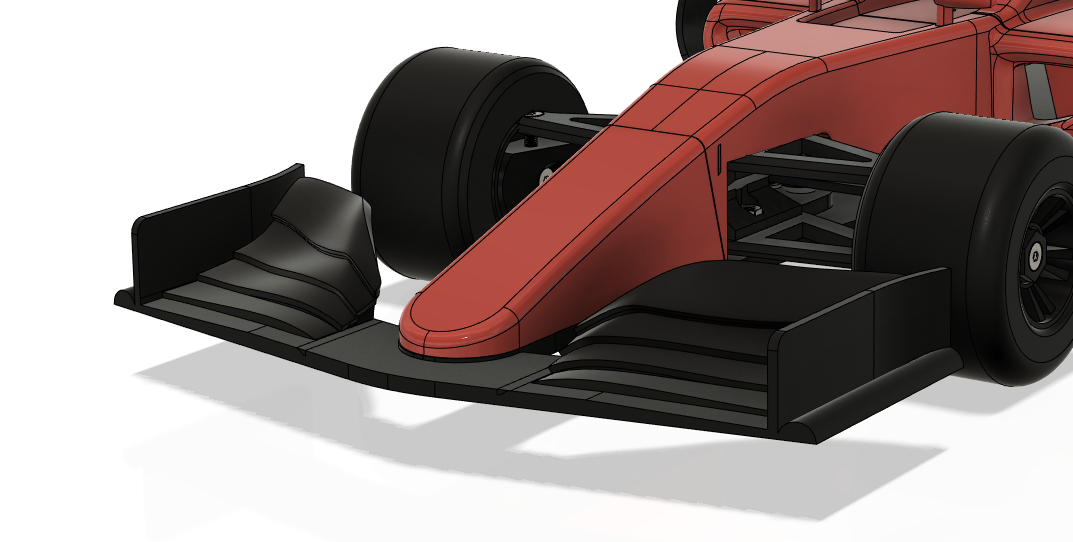
These Machine Learning-driven approaches combine supervised learning techniques with optimization algorithms to create hybrid solutions that can handle the uncertainty in real-world engineering problems and the constraints typical in engineering design.

How does machine learning optimization work?

Machine Learning Optimization refers to the process of improving the performance of machine learning models. It works on four aspects:

1. tuning the model’s hyperparameters
2. selecting appropriate features
3. choosing the model architecture
4. optimizing the training process

The goal is to enhance accuracy, reduce overfitting, and shorten training time, improving the machine learning algorithm’s performance on its task.

Hyperparameters are settings chosen before training a machine learning model, unlike parameters, which the model learns from data. These settings control aspects such as model complexity and learning efficiency, thereby influencing performance. Proper tuning of hyperparameters can reduce prediction errors by ensuring the model generalizes well to unseen data. For example, the learning rate in a neural network (NN) determines how much model weights adjust per iteration. A high rate causes instability, while a low rate slows convergence.

Machine Learning Optimization techniques are crucial for making accurate predictions or decisions during model training. Hyperparameter tuning is essential in model optimization, and the approaches differ in cost and efficiency:

• Random and grid searches are straightforward but can be computationally expensive.
• More advanced techniques, such as Bayesian optimization or gradient-based tuning, improve efficiency and performance.

These techniques aim to minimize a specific function, called the loss or cost function. Generally, a cost function (or objective function) C measures how good or bad a solution is. For example, it might measure a model’s prediction error.

Each method is suited to different scenarios, depending on the nature of the data, the model’s architecture, and the available computational resources. The choice of optimization method can significantly affect the training speed, the quality of the final model, and its ability to generalize.

Before optimization, data preprocessing, including feature scaling, is crucial to ensure that input parameters contribute proportionally to the optimization process. This step improves the stability of surrogate models like Gaussian Processes and Deep Learning-based approaches, leading to more accurate design predictions.

The gradient descent method

Let’s use the gradient descent method to understand the basic mathematics of optimization, which applies to machine learning and engineering problems. Gradient Descent is one of the first-order optimization algorithms used in machine learning and is an iterative method for finding a local minimum of a differentiable multivariate function.

The variable x represents what we can control:

• In Machine Learning, x might be model weights
• In engineering, x might be the shape parameters of a wing

The loss landscape is like a terrain map showing how the cost (introduced previously) C varies with x. Imagine hiking in the mountains: Height represents the cost C, our position represents parameters x, and we want to find the lowest point (minimum).

The gradient indicates the direction in which the function increases the fastest at our current position.

This leads to the gradient descent update rule:

Δx = −η ∇C

where Δx denotes the change in x, η is the learning rate that controls the step size, and the negative sign indicates that we move in the direction opposite to the gradient. This process is repeated until we converge to a minimum of C. Iterative optimization involves comparing the model’s output with the expected results after each iteration.

On the learning rate

The learning rate η is a crucial hyperparameter in gradient descent. It controls the step size for each parameter update and determines how aggressively the model moves toward minimizing the cost function C at each iteration.

• With a small learning rate (η too low), the machine learning model updates parameters in very small steps, leading to slow convergence. If there is insufficient momentum, it may take too many iterations to reach the minimum or get stuck in a local minimum.
• With a high learning rate (η too high), the model takes big steps, which can cause it to overshoot the minimum and oscillate without settling. The loss might even diverge in extreme cases of large learning rates, preventing convergence.

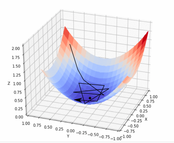
Some optimization techniques, such as Adam and RMSprop, dynamically adjust the learning rate during training. These methods start with larger steps and refine them as training progresses, balancing speed and stability.

Choosing an optimal learning rate is key to using a training dataset to get the most accurate model.

A common strategy is to start with a moderate value of learning rate (e.g., 0.01 for many problems) and decay it over time to fine-tune the solution as the model nears convergence.

Loss landscape and gradient descent

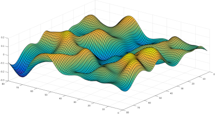
A loss landscape shows how a model’s loss varies with its parameters. Each set of parameter values has a height equal to its loss, so the result is a surface, and training looks for the lowest point on it.

For a house-price model, the loss at any given setting is the gap between predicted and actual prices across the data, using inputs such as size, number of bedrooms, and location.

Gradient descent moves across the surface by following the negative gradient, updating parameters until the loss stops falling or a stopping criterion is met.

Momentum and adaptive learning rates adjust the step size over time, thereby accelerating convergence and reducing the risk of settling into a shallow local minimum.

The shape sets the difficulty: a single global minimum is easy to reach, while many local minima give the optimizer more places to stop early.

Stochastic Gradient Descent is an extension of gradient descent that introduces randomness to speed up convergence and reduce memory usage. Stochastic Gradient Descent computes the gradient and updates the model parameters for each training example, either individually or in small batches.

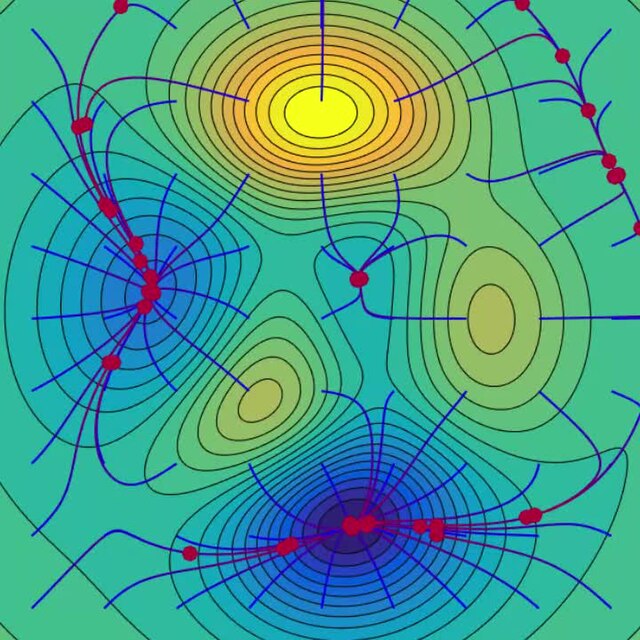
Adaptive learning rate methods: Adagrad, RMSprop.

Adagrad adapts the learning rate for each parameter, giving larger updates for infrequent parameters and smaller ones for frequent ones.

RMSprop modifies Adagrad by normalizing the gradient using a moving average of squared gradients, preventing the learning rate from decreasing too rapidly.

Objective functions: ADAM

ADAM (Adaptive Moment Estimation) is a popular optimizer for training deep NNs. It is particularly effective in high-dimensional, complex loss landscapes. ADAM updates model parameters like gradient descent but adapts the learning rate (η) for each parameter based on historical gradients, improving stability and convergence. Adam is an optimization algorithm that combines ideas from momentum optimization and RMSprop.

Adam is noted for its efficiency at handling sparse gradients, making it suitable for tasks such as natural language processing.

Bayesian optimization

Bayesian optimization provides a rigorous framework for optimizing expensive-to-evaluate objective functions f(x) by maintaining and updating probability distributions over candidate solutions. The method constructs a probabilistic surrogate model (typically a Gaussian Process) that captures both the predicted value μ(x) and the uncertainty σ(x) at any point x in the search space. Bayesian optimization iteratively improves the model by refining hyperparameters based on previous results.

Metaheuristic optimization algorithms

Metaheuristic optimization algorithms guide lower-level heuristic techniques in optimizing complex search spaces. Many are inspired by natural behaviors, such as genetic algorithms that mimic evolution or particle swarm optimization that follows bird flocking. In evolutionary algorithms, each iteration of a hyperparameter value is assessed and combined with other high-scoring hyperparameter values.

Evolutionary algorithms: genetic algorithms

Genetic algorithms optimize by mimicking natural evolution, using selection to identify solutions. These solutions form a population that is evaluated by an objective function. The best chromosomes reproduce, generating new solutions through combination and mutation until a satisfactory solution is found. Genetic algorithms can be computationally demanding.

Swarm intelligence

Swarm intelligence algorithms emulate the collective behavior of organisms to solve optimization problems. The key insight is that simple individual behaviors can create sophisticated collective problem-solving abilities.

• Particle swarm optimization simulates bird flocking. The core principle is simple: particles adjust their velocities based on their own and their neighbors’ successful experiences. 
• Ant Colony Optimization mimics how ants find food using pheromone trails. As more ants choose better paths, these trails strengthen. In the algorithm, virtual ants deposit more pheromones on better solutions, allowing the best paths to accumulate the strongest pheromone levels over time.
• The Artificial Bee Colony algorithm mimics how honeybees find nectar. The algorithm uses different types of bees: employed bees stick with known food sources, onlookers choose sources based on their quality, and scouts search for new sources.

How to create an optimal shape: machine learning-based optimization examples

Designing industrial objects optimizes shapes for performance, materials, and manufacturability via CAD. For instance, optimizing a car’s rear window for aerodynamics or a lightweight bracket for fatigue resistance requires simulations. CAE simulations assess performance in fluid dynamics or structural analysis, but they may take weeks and demand high computing power.

Companies can enhance CAE by investing in High-Performance Computing (HPC), using GPUs for parallel processing, or, most efficiently, applying AI for real-time simulations.

Deep neural networks

Computer-aided engineering (CAE) limits analyses to a few per day due to computational demands, underscoring the need for real-time alternatives such as physics-aware AI models. Deep learning facilitates this through physics-aware AI models; techniques such as Neural Concept identify geometric features using NNs. AI and data science are intertwined, as AI creates predictive models from consistent datasets such as temperature and pressure. NNs minimize prediction errors and link design with performance goals.

Deep learning (DL) relies on data, as training data influences the model’s ability to recognize patterns and make predictions. More data typically enhances performance, but data quality is vital; poor or biased data can undermine results. Unlike traditional AI systems focused on rule-based decisions, DL excels at predictions, leaving final decisions to users, even as optimization capabilities evolve.

Why is data important for training?

Training data impacts model performance, generalization, and accuracy. High-quality, diverse data helps models recognize patterns, reduce bias, and make reliable predictions. In contrast, poor data can result in overfitting, underfitting, or biased outputs, hindering real-world use.

For instance, convolutional neural networks (CNNs) trained on a limited number of medical images may not generalize to new scans, compromising diagnostic reliability. Similarly, self-driving car models trained solely on sunny conditions may struggle in rain or snow. While large datasets enhance performance, when data is scarce, we can implement strategies such as synthetic data, transfer learning, and data augmentation.

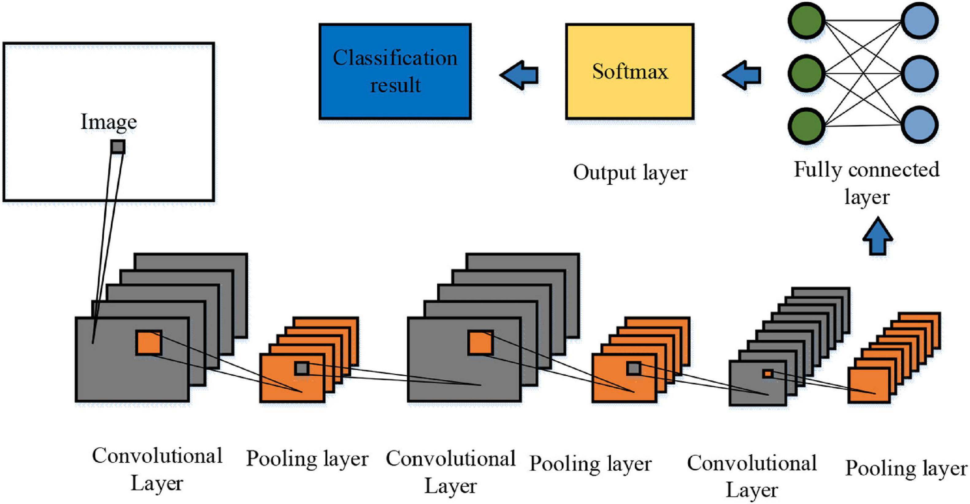
CNNs are particularly relevant in engineering applications because they can process and analyze complex image-based data. Their strength lies in extracting spatial features from 2D images, 3D models, and CAD designs, making them highly effective for engineering tasks.

Many believe that deep learning requires millions of samples, but industrial applications such as defect detection have succeeded with only a few hundred labeled cases through iterative model refinement. Initial data from past designs can significantly reduce future data requirements in CAD engineering simulations.

Engineering optimization

Testing new designs through simulations is time-consuming and costly. Design spaces have many dimensions, such as material properties and performance metrics, making manual optimization impractical. For example, optimizing a car’s aerodynamics involves tuning interrelated parameters like shape and material composition. We need a constrained optimization algorithm that balances the objectives of structural strength, weight reduction, and energy efficiency, satisfies equality or inequality constraints in design problems (including material and manufacturing cost limits), and handles convex constraints in non-convex optimization scenarios where escaping saddle points matters. The next section will explore efficient methods for industrial design optimization.

What are the classic requirements for optimization methods?

Optimization theory examines algorithms and strategies for identifying the optimal solution to a problem. Optimization techniques are frequently applied in engineering to develop systems or processes that function efficiently and effectively.

Objective functions in deep learning

In Supervised Learning, artificial NNs aim to minimize a cost function C using known data. The cost function is the difference between the NN’s prediction ŷ and the actual solution y and is also a function of the inputs x.

Therefore, C = C(x;y,ŷ) over the entire dataset. The concept works statistically across a whole dataset composed of samples, each with its own loss (i.e., the deviation of a single data point), whereas the cost is the sum of all data points.

The minimum of this function is the artificial NN’s learning solution.

There are several ways to express the cost function mathematically, and a few of them are listed here:

• Mean Absolute Error (MAE) is a loss function used in regression problems by taking the mean of the absolute differences between the predicted and actual values.
• Mean Squared Error (MSE) squares the individual errors rather than taking their absolute values.
• Root Mean Squared Error (RMSE) is computed by taking the square root of the MSE.
• R² score indicates the proportion of the variance in a regression model’s response variable that the predictor variables explain. The higher the R² value, up to a maximum of 1, the better a model fits a dataset.

Cost functions can be managed because supervised learning provides a known solution. Thus, one predictive model can outperform another due to better predictions.

Both learning and achieving better designs are optimization problems: supervised learning aims for predictive accuracy, while design optimization seeks the best design given specific performance objectives and constraints.

How to optimize 3D shapes

Starting with a digital product shape in CAD, which algorithmic options help designers optimize functional requirements such as weight and mechanical robustness? Standard methods connecting CAD to optimization algorithms include:

1. Topology optimization uses simulations to determine optimal material distribution subject to constraints such as stress and displacement, producing lightweight designs. But it is case-specific and inflexible. Machine learning-based optimization, by learning patterns, generalizes across designs.

2. Parametric design enables easy adjustments by varying parameters and typically works across different processes or materials, though it raises questions about whether the results are truly optimal or merely improved.

3. Shape optimization is more flexible than parametric design, using algorithms to improve shapes, reduce drag, increase stiffness, and allow free-form deformation without added constraints.

The idea now is to train the artificial NN in the AI software to yield, for example, the hydrodynamic coefficients of a wing. The three-dimensional optimization based on machine learning is performed on meshes whose shapes evolve at each iteration until they reach an optimal form under the given constraints.

Applications of machine learning-based optimization: case study

We will now examine an example of AI use in mechanical engineering: how machine learning optimizes aerodynamic profiles in aerospace design. The focus is not on the machine learning model and its hyperparameter optimization, and the collaboration between data scientists and engineers is oriented toward a better-performing industrial design enabled by an accurate Machine Learning/Deep Learning model.

The project sought to meet a UAV’s aerodynamic and geometric requirements while optimizing performance. The algorithm aligned engineering outcomes with actual needs. The optimization process relied on simulation software (CAE) to evaluate UAV performance across configurations and inform design decisions.

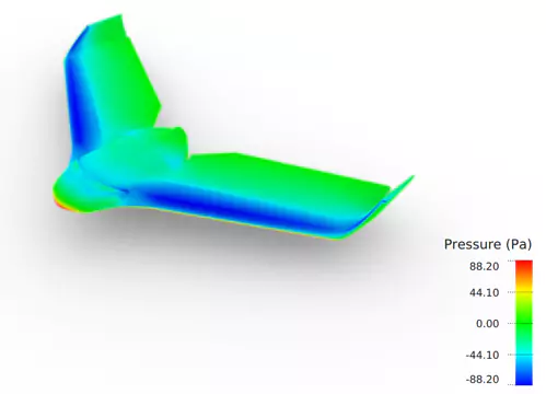
Neural Concept streamlined simulations into AI predictions, exploring and optimizing drone aerodynamics using three CFD simulation levels:

• a rough (low fidelity) estimate,
• an AirShaper concept simulation,
• A detailed simulation, capped at 50 iterations, was used to enhance the design.

Low-fidelity CFD and a pre-trained NN aided in innovative design exploration. The goal was to enhance the lift-to-drag (L/D) ratio crucial for UAV autonomy, and optimization iterations monitored L/D efficiency.

The framework started with low-accuracy simulations for pre-training and was refined with high-accuracy simulations.

This approach increased the L/D ratio by 4.25% and reduced drag by 6.25%, thus providing an optimal combination.

Key takeaways

• Machine learning optimization splits into optimizing the model (hyperparameters, architecture, training) and optimizing a physical design with a trained model.
• Gradient descent minimizes a cost function by stepping opposite the gradient; the learning rate sets the step size and governs convergence speed and stability.
• Adaptive optimizers (Adam, RMSprop, or Adagrad) adjust the learning rate per parameter, which helps in high-dimensional, non-convex landscapes.
• Metaheuristics such as genetic algorithms and particle swarm optimization search design spaces where gradients are unavailable or unreliable.
• A predictive model trained on past simulations replaces costly CFD or FEA runs during optimization, enabling an engineer to evaluate more designs per day.
• Training data quality governs accuracy; industrial cases such as defect detection have succeeded with a few hundred labeled examples seeded by earlier designs.
• In the case study, the method matched CFD ground truth and improved a UAV’s lift-to-drag ratio by 4.25%.

FAQ

Is supervised learning similar to design optimization?

Unlike design optimization, which seeks the best solution under constraints, Supervised learning aims to minimize a cost function based on known solutions. However, both are optimization problems that seek optimal outcomes.

What are the challenges associated with optimization in deep learning?

High computational demand, risk of overfitting, and navigating complex loss landscapes.

How do optimization algorithms differ between supervised and unsupervised learning?

Supervised learning uses labeled data to minimize error; unsupervised learning focuses on data structure without labels.

What is the role of hyperparameters in machine learning models?

Control model behavior, complexity, and the learning process; not learned from data.

How do I tune hyperparameters to improve machine learning model performance?

Start with a coarse search over the hyperparameters that most affect the loss, usually learning rate, regularization strength, and model capacity. Grid search and random search establish a baseline. Bayesian optimization then concentrates evaluations where the model predicts improvement, which reduces the number of expensive training runs. Validate every configuration on held-out data so gains reflect generalization rather than fit to the training set.

How can I reduce overfitting while optimizing my machine learning model?

Add regularization that penalizes large weights (L1 or L2), apply dropout to neural networks, and stop training when validation loss no longer decreases. More or more diverse training data reduces overfitting directly. Cross-validation shows whether a configuration generalizes before you commit compute to full training.

How do grid search and Bayesian optimization compare for hyperparameter tuning?

Grid search evaluates every combination on a fixed lattice, so cost grows exponentially with the number of hyperparameters and much of the search covers poor regions. Bayesian optimization builds a probabilistic model of the objective and selects the next configuration with the greatest expected improvement, achieving comparable results in far fewer evaluations. Grid search stays reasonable for two or three low-cardinality parameters, while Bayesian optimization pays off when each training run is expensive.

How do AutoML tools compare to manual hyperparameter tuning?

AutoML automates model selection, hyperparameter search, and feature preprocessing, which shortens the path to a working baseline and lowers the expertise required. Manual tuning keeps an advantage when domain knowledge constrains the search or when the objective includes requirements AutoML does not encode, such as inference latency or interpretability. Many engineers use AutoML to reach a starting point, then refine by hand.

How does stochastic gradient descent compare to batch gradient descent for large datasets?

Batch gradient descent computes the gradient over the full dataset before each update, which is accurate but memory-bound and slow on large data. Stochastic gradient descent updates on one example or a small mini-batch, so it uses less memory and starts improving the model sooner. Its update noise can help the optimizer escape shallow local minima. Mini-batch sizes between 32 and 512 balance update stability against throughput on most hardware.

When should I use second-order optimizers like L-BFGS instead of first-order methods?

Second-order methods use curvature information to take better-scaled steps and converge in fewer iterations on smooth, moderately sized problems. L-BFGS is well-suited to deterministic objectives with up to a few thousand parameters, such as classical regression or physics-based fitting. First-order methods such as SGD and Adam stay the default for deep networks, where the parameter count and gradient noise make full curvature estimates impractical.

How does feature engineering improve machine learning pipeline optimization?

Feature engineering transforms raw inputs into representations that expose the structure a model needs, thereby reducing the capacity and data required to achieve a given accuracy. Scaling and encoding keep inputs on comparable ranges so gradient-based training converges reliably. In engineering problems, physics-derived features, such as dimensionless ratios,  carry more signal than the raw measurements.

How do model compression, pruning, and quantization optimize inference performance?

Pruning removes weights or channels that contribute little to the output, thereby shrinking the model and reducing its compute cost. Quantization stores and computes weights in lower-precision formats, reducing memory traffic and latency on supported hardware. Compression combines these with methods such as knowledge distillation, where a smaller model learns to reproduce a larger model’s outputs. Each step trades a controlled amount of accuracy for faster, cheaper inference.

How does optimization work in reinforcement learning?

In reinforcement learning, algorithms are optimized by maximizing cumulative rewards.

How do you improve a model’s accuracy and generalization?

Regularization techniques improve model generalization by penalizing complex weights, and ensemble methods enhance accuracy by combining predictions from multiple models.

How do you prepare data before training a model?

Data cleaning addresses noise and class imbalances in datasets, and dimensionality reduction techniques such as PCA retain the most informative variance by projecting data onto principal components.

How do you reduce model latency at inference?

Quantization converts model weights to lower-precision formats to reduce latency.

How is optimization applied beyond model training?

Dynamic pricing uses optimization algorithms to maximize revenue and minimize costs.

‍